The Hidden Data-Engineering Work Behind Real-Time Drilling Analytics

A drilling model may be expressed in a few equations, but producing trustworthy real-time inputs for that model requires synchronization, tag mapping, context management, data-quality checks, depth alignment, buffering, provenance, and careful handling of stale or missing information.

A drilling dashboard might show:

• ROP,
• WOB,
• RPM,
• torque,
• standpipe pressure,
• MSE,
• modeled ECD,
• rig state.

To the user, those values may appear together on one screen as though they came from one coherent dataset.

They usually did not.

One channel may originate from the rig control system.

Another may arrive through an EDR.

Another may come through WITS or WITSML.

Mud properties may have been entered manually.

The active BHA may come from a reporting database.

Survey information may arrive independently.

Formation information may come from yet another system.

Some values update ten times per second.

Others once per second.

Others every few minutes.

Some change only when a person edits a report.

The analytical model at the end of this chain may be elegant.

Getting the correct data into that model at the correct time is often the harder engineering problem.

Published real-time drilling systems make this clear.

SPE-191797 describes the first prerequisite for drilling optimization and automation as a reliable data-acquisition and handling system capable of receiving different-frequency data across multiple platforms while maintaining data quality.[1]

The field architecture described in that work integrated several protocols and sources, including high-frequency PLC data, WITS0, WITSML, OPC-connected devices, mudlogging information, and contextual information from the daily drilling report.[1]

SPE-191426 similarly states that real-time torque-and-drag analysis requires the ability to receive data at different frequencies and combine live measurements with contextual information such as:

• BHA,
• wellbore geometry,
• trajectory,
• mud properties.[2]

These are not peripheral software concerns.

They determine what the engineering model actually thinks the well looks like.

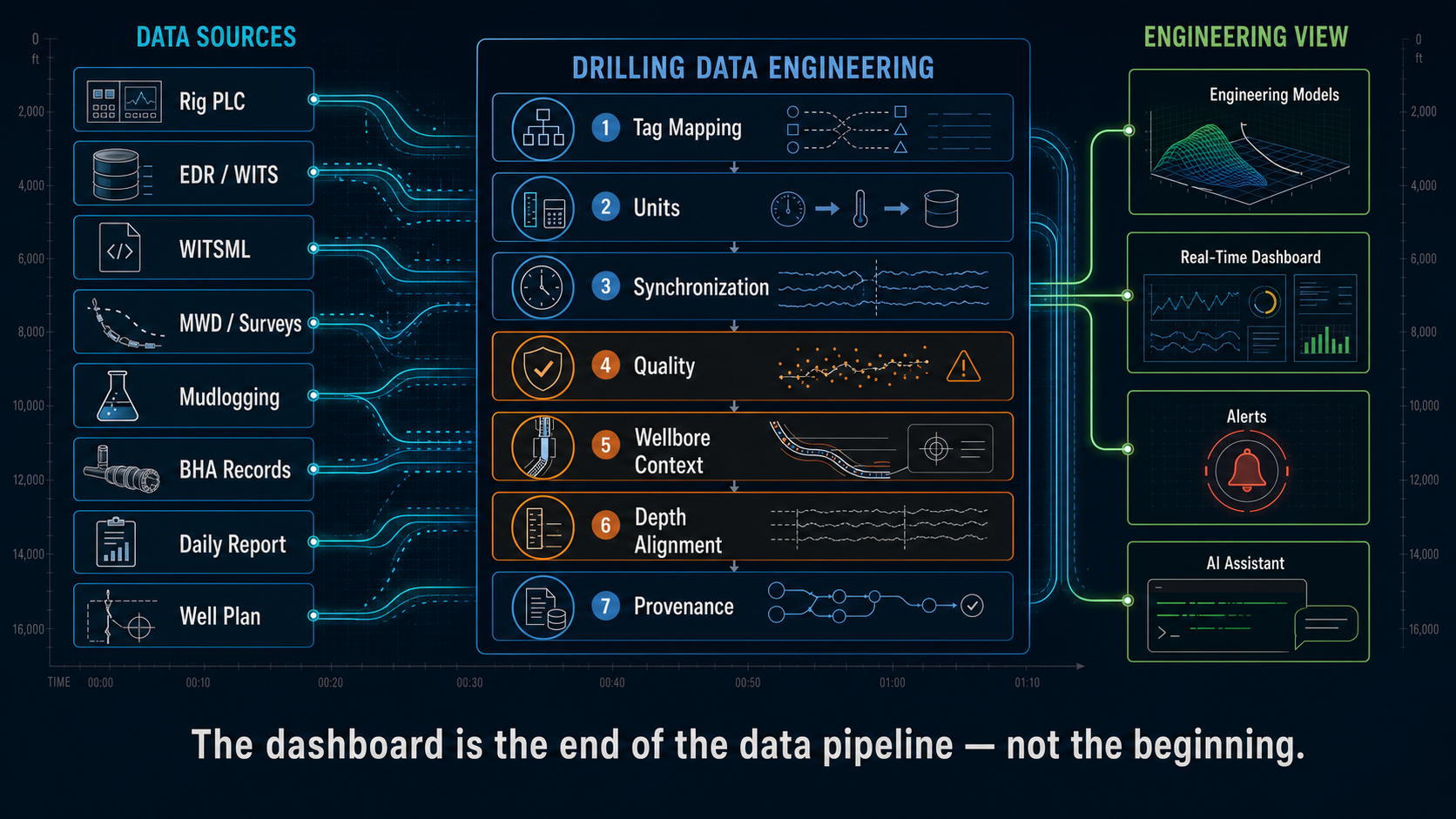
A real-time dashboard is the end of the drilling-data pipeline—not the beginning.

The Rig Does Not Produce One Dataset

It is tempting to talk about:

the rig data.

Operationally, there are usually several datasets.

Examples can include:

Rig-control data

• block position,
• hook load,
• RPM,
• torque,
• pump strokes,
• pressure.

EDR data

A selected set of surface channels, often exposed through industry-standard or vendor interfaces.

Directional data

• surveys,
• inclination,
• azimuth,
• toolface.

Mud data

• mud weight,
• PV,
• YP,
• gel strengths,
• temperature-dependent properties where available.

BHA and drillstring context

• bit,
• motor,
• stabilizers,
• drillpipe,
• dimensions.

Well architecture

• hole size,
• casing depth,
• casing ID,
• wellbore trajectory.

Operational reporting

• BHA changes,
• casing runs,
• mud changes,
• daily activities,
• operational notes.

Real-time analytics needs to convert those sources into one coherent representation.

That is fundamentally a data-engineering task.

Transporting a Number Is Not the Same as Understanding It

Suppose a stream contains:

RPM = 120

Several questions remain.

Is that:

• surface RPM?
• bit RPM?
• motor RPM?
• commanded RPM?
• actual measured top-drive RPM?

Now consider:

DEPTH = 14,200

Is that:

• hole depth?
• bit depth?
• measured depth?
• TVD?

A communication protocol can successfully transport the value:

14,200

without resolving its engineering meaning.

This is an important limitation to understand when working with WITS, WITSML, APIs, or any other data interface.

Successful data transmission does not guarantee semantic correctness.

Tag Mapping Is an Engineering Problem

Different rigs and vendors may expose conceptually similar measurements under different:

• tag names,
• channel identifiers,
• units,
• scaling conventions.

A generic analytics model wants something conceptually simple:

$$Torque_{surface}$$

But Rig A might expose one tag.

Rig B another.

Rig C may expose two torque measurements from different systems.

SPE/IADC-184743 describes the use of rig-specific mapping layers so that different sensor types and tags can feed a common data model without rewriting the analytical model for each rig.[3]

That abstraction is essential for fleet-scale analytics.

Conceptually:

$$Rig\ Specific\ Tag \rightarrow Canonical\ Engineering\ Variable$$

For example:

$$VendorTag_A \rightarrow SURFACE_TORQUE$$

Once that mapping is wrong, everything downstream can still execute perfectly.

It will simply calculate the wrong thing.

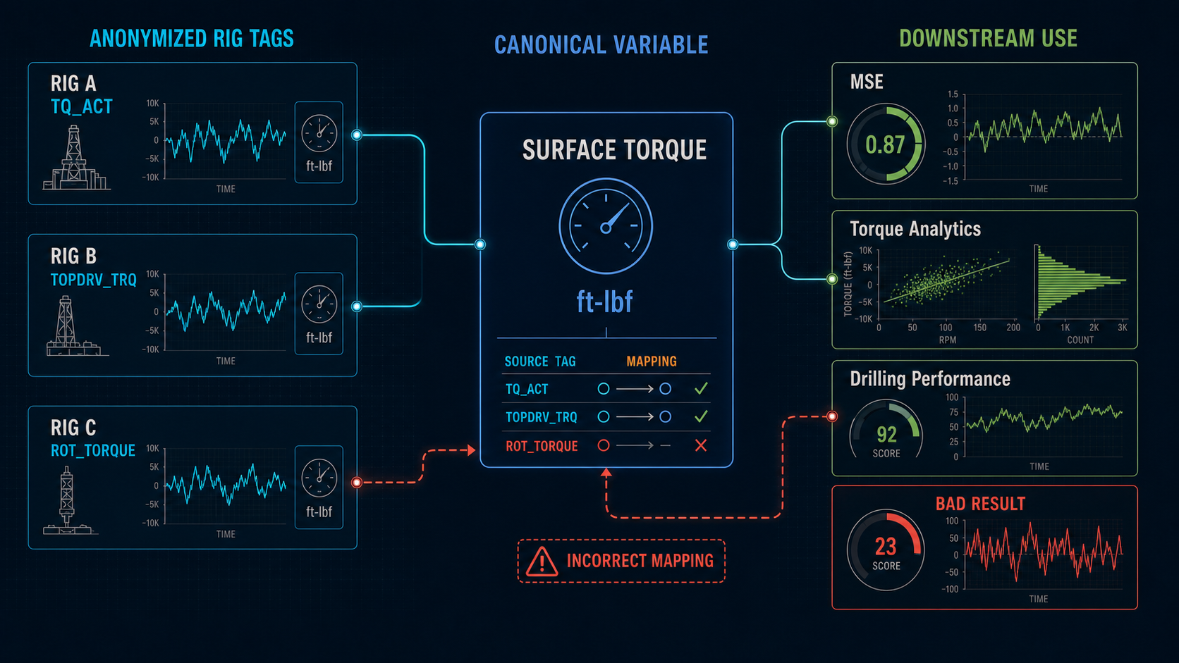
Tag mapping converts rig-specific names into engineering variables; a wrong map propagates into every dependent calculation.

Units Need the Same Treatment

Suppose one source reports torque in:

ft-lbf

and another in:

kft-lbf.

Or pressure in:

• psi,
• kPa.

Or depth in:

• feet,
• meters.

The database can accept all of them as floating-point numbers.

The engineering equation cannot.

A robust data model therefore needs explicit unit metadata and normalization.

Conceptually:

$$Raw\ Value + Raw\ Unit \rightarrow Canonical\ Value + Canonical\ Unit$$

Unit conversion should happen deliberately and reproducibly.

A unit should not be inferred from:

• magnitude,
• rig name,
• what the programmer remembers about one vendor.

Time Is the First Common Coordinate

Real-time sensor streams usually arrive with timestamps.

That gives us a common coordinate:

$$t$$

But different sources may update at:

• 10 Hz,
• 1 Hz,
• 0.1 Hz,
• irregular intervals.

SPE-191426 and SPE-191797 both emphasize the challenge of combining data with different frequencies.[1,2]

Suppose at:

10:00:00

we have torque.

At:

10:00:00.4

we have RPM.

At:

10:00:01

we have ROP.

Which values belong in one MSE calculation?

The software must define an alignment strategy.

That might involve:

• nearest observation,
• bounded forward fill,
• resampling,
• interpolation,
• aggregation.

That decision is part of the analytical method.

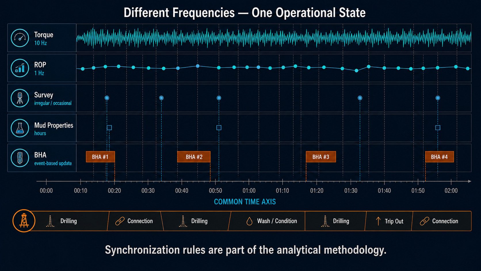
Synchronization rules are part of the analytical methodology.

Timestamp Equality Is Not the Same as Physical Simultaneity

Two database rows may both say:

10:00:00

but the measurements may have travelled through different:

• devices,
• acquisition systems,
• buffers,
• communication links.

If one stream has two seconds of latency, a perfectly executed timestamp join may still align different moments in the physical process.

This matters when studying sequence.

For example:

Did:

• WOB change,
• then torque,
• then ROP?

Or did the apparent sequence result from stream latency?

As analytics becomes more sensitive to short events, synchronization quality becomes increasingly important.

Data Freshness Is Different From Data Availability

Suppose the latest mud weight in the database is:

12.1 ppg.

The value exists.

Is it current?

Perhaps it was entered:

six hours ago.

The well may have been weighted up since then.

Likewise, the database may contain:

• a BHA,
• a survey,
• casing depth.

But the relevant question is:

Is this the latest valid context for the operation being analyzed?

This is why real-time systems need more than:

$$value$$

They also benefit from:

$$value + timestamp + source + quality$$

A stale value is not equivalent to a newly observed value with the same number.

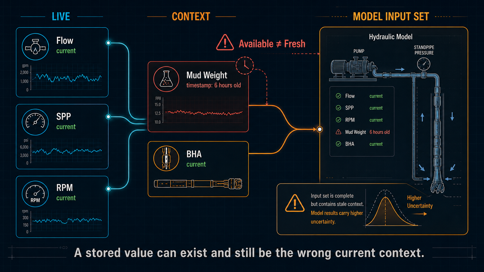
Available data is not necessarily fresh data.

Contextual Data Can Be Wrong Even When the Sensor Data Is Perfect

Imagine surface measurements are excellent.

The hydraulic model receives:

• accurate flow,
• accurate SPP,
• accurate RPM.

But the BHA record contains:

the previous bit nozzle configuration.

The model predicts the wrong pressure.

Measured pressure now disagrees with modeled pressure.

An event detector may conclude:

something changed hydraulically.

The actual problem is contextual data.

SPE-181076 describes exactly this class of challenge: well and rig information needed by analytical models was sometimes entered incorrectly or unavailable, which then affected model predictions. The paper also notes that context updates can lag the real operation when humans are involved.[4]

This leads to an important rule:

Context quality is data quality.

Context Is Not Merely Metadata

In ordinary software, metadata may describe a dataset without changing its numerical interpretation.

In drilling, contextual information frequently enters directly into the physics.

Consider a hydraulic model.

Inputs may include:

• hole size,
• drillpipe ID/OD,
• BHA geometry,
• nozzle area,
• mud rheology.

Change any of those and the predicted pressure changes.

Consider torque and drag.

Inputs include:

• trajectory,
• pipe weights,
• casing depth,
• BHA,
• mud weight,
• friction factors.

Context is therefore not decorative information around the sensor stream.

It is part of the mathematical state of the well.

Context Also Changes Over Time

A common data-modeling mistake is to store:

the BHA

as though a well had only one.

Real wells have:

• multiple BHA runs,
• bit changes,
• motor changes,
• casing strings,
• mud-property changes.

The correct question is not:

What is the BHA for this well?

It is:

Which BHA was active at this time and depth?

Conceptually:

$$Context = f(Time,Depth)$$

The same applies to:

• casing state,
• mud properties,
• active wellbore.

Historical analytics becomes unreliable if present-day context is applied retroactively to older data.

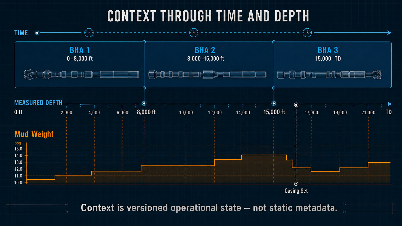
Context is versioned operational state—not static metadata.

Sidetracks Make the Data Model Harder

Measured depth alone does not uniquely identify a physical location when multiple wellbores exist.

Imagine:

Main bore

14,000 ft MD

Sidetrack

14,000 ft MD

Those represent different physical locations and drilling histories.

Therefore:

$$Well + MD$$

may not be enough.

The analytical key may need something closer to:

$$Well + Wellbore + MD$$

This is especially important when retrieving:

• surveys,
• plans,
• BHA records,
• offset intervals.

Without wellbore identity, perfectly valid data can be attached to the wrong trajectory.

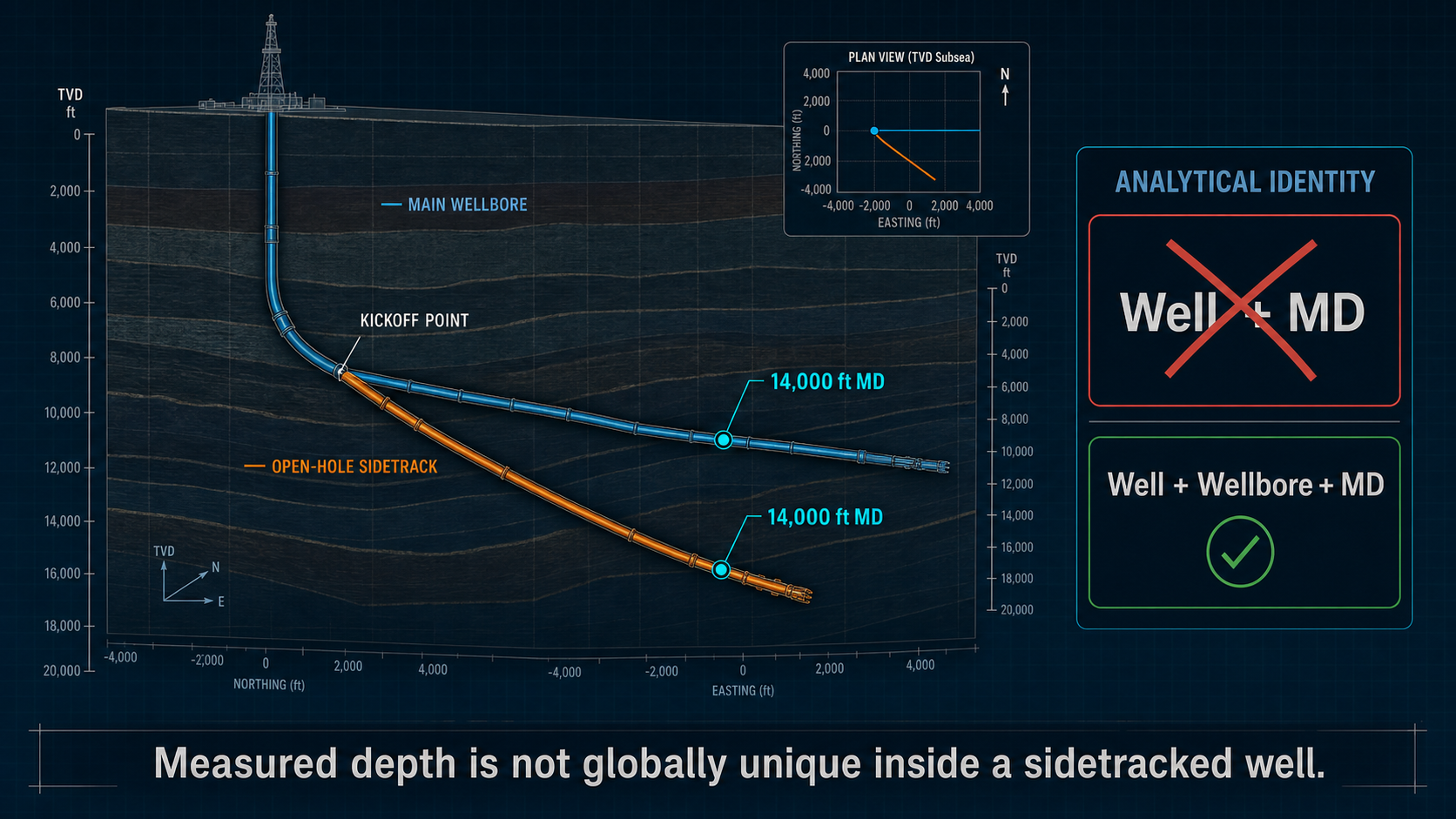
Measured depth is not globally unique inside a sidetracked well.

Time and Depth Need to Be Linked

The earlier article on time- and depth-based analytics explained why the two domains answer different questions.

Data engineering has to create the bridge between them.

A real-time sensor sample begins naturally as:

$$(timestamp,value)$$

To plot it against depth, the system needs an appropriate depth value for that instant.

But even “depth” is ambiguous.

Possible coordinates include:

• hole depth,
• bit depth,
• TVD,
• formation-relative depth.

The transformation should therefore be explicit.

A system should not merely add a column named:

depth

and assume the ambiguity disappeared.

Hole Depth and Bit Depth Cannot Be Interchanged

During drilling:

$$Bit\ Depth \approx Hole\ Depth$$

much of the time.

During a trip:

hole depth is fixed while bit depth changes dramatically.

During reaming:

bit depth changes without necessarily creating new hole.

A depth transformation based on the wrong coordinate can make an operational event appear at the wrong physical location.

This is one reason rig state, depth semantics, and data engineering are tightly connected.

Rig State Becomes a Data-Transformation Variable

Rig-state classification is usually described as an analytical product.

It is also a data-engineering tool.

Suppose we want:

rotary ROP distribution.

We first need to select:

rotary drilling observations.

Suppose we want:

pick-up hook-load calibration.

We need:

pick-up observations.

Suppose we want:

connection time.

We need:

connection boundaries.

Therefore:

$$Raw\ Stream \rightarrow Rig\ State \rightarrow Analytical\ Population$$

The rig-state output becomes part of how the dataset itself is organized.

Data Quality Should Occur Before Sophisticated Analytics

SPE-181076 emphasizes the operational cost of bad drilling data.

Its field trial focused on eight core surface channels and established a workflow to identify and improve:

• missing data,
• outliers,
• bias errors.[5]

This order matters.

Consider MSE.

A sophisticated MSE algorithm operating on a bad torque sensor simply creates a sophisticated wrong answer.

The same applies to:

• torque and drag,
• hydraulics,
• dysfunction detection,
• machine learning.

There is little value in improving the downstream model while ignoring upstream measurement quality.

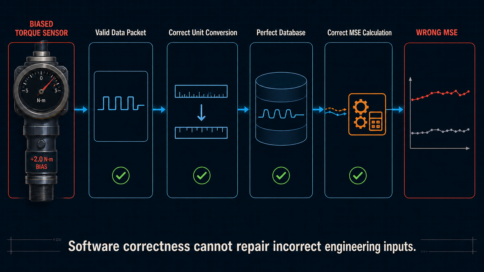
Software correctness cannot repair incorrect engineering inputs.

Quality Needs More Than a Null Check

It is relatively easy to detect:

• missing value,
• impossible value.

Bias is harder.

Suppose torque reads:

14,000 ft-lbf

when the correct value is:

10,000 ft-lbf.

Fourteen thousand may be entirely plausible numerically.

A simple range check will pass it.

This is why drilling-data validation can use redundancy among:

• related sensors,
• process expectations,
• physical models.

The data-quality problem is therefore itself an engineering-analysis problem.

Source Provenance Should Survive Every Transformation

Suppose a dashboard shows:

ECD = 12.4 ppg

Where did that number come from?

Was it:

• PWD measured,
• surface-calculated,
• hydraulic-model output,
• manually entered?

A useful data architecture should preserve that distinction.

Likewise, consider:

WOB = 35 klbf

Was it:

• rig-reported surface WOB,
• recalculated surface WOB,
• modeled downhole WOB?

The numeric value alone is incomplete.

A robust derived-data record should conceptually retain:

• source,
• calculation method,
• timestamp,
• inputs,
• version where appropriate.

This becomes increasingly important once AI systems begin consuming the same data.

Derived Values Need Lineage Too

Imagine an engineer asks:

Why was MSE high at 15,300 ft?

To answer properly, the system may need to reconstruct:

• torque used,
• WOB used,
• RPM used,
• ROP used,
• bit size,
• calculation version,
• rig state.

If those relationships are not preserved, the final KPI becomes difficult to audit.

A general pattern is:

$$Measurement \rightarrow Cleaned\ Measurement \rightarrow Derived\ Feature \rightarrow Model\ Output \rightarrow Recommendation$$

Each layer should retain enough lineage to trace backward.

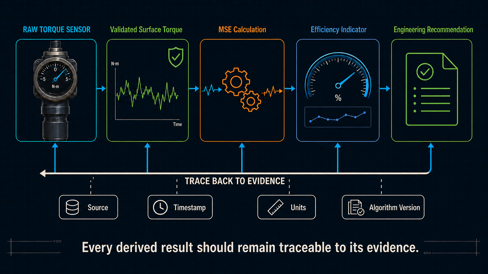
Every derived result should remain traceable to its evidence.

Late-Arriving Data Creates Another Problem

Suppose a survey is not available in real time.

A torque-and-drag calculation runs using the last available trajectory.

Two hours later, the new survey arrives.

Now we have two possible historical truths:

What the model knew at the time

and:

What we know now with corrected context.

Both can be valuable.

For operational audit, we may want:

the information available when the decision was made.

For post-well analysis, we may want:

the best corrected historical dataset.

A mature data architecture may therefore distinguish:

• event time,
• ingestion time,
• revision/version.

Historical Data Should Not Quietly Rewrite Operational History

Suppose a mud-property record is corrected after the well.

If the historical model outputs are recomputed automatically, a later engineer may see a result that differs from what the rig saw in real time.

That may be desirable for:

post-well normalized analysis.

It is undesirable if the question is:

Why did the engineer make this decision at 2 PM Tuesday?

Reproducibility requires knowing which version of the inputs was available at the time.

Connectivity Cannot Be Assumed

Rig connectivity can be intermittent.

SPE-191797 describes local storage and store-forward capability so rig data could be retained and later transferred to the office when telecommunications were interrupted.[1]

That design principle remains important.

A real-time system should distinguish:

remote connectivity failed

from:

rig acquisition failed.

Where practical, local acquisition allows:

• the rig to continue analyzing data,
• the complete record to be preserved,
• the office copy to catch up later.

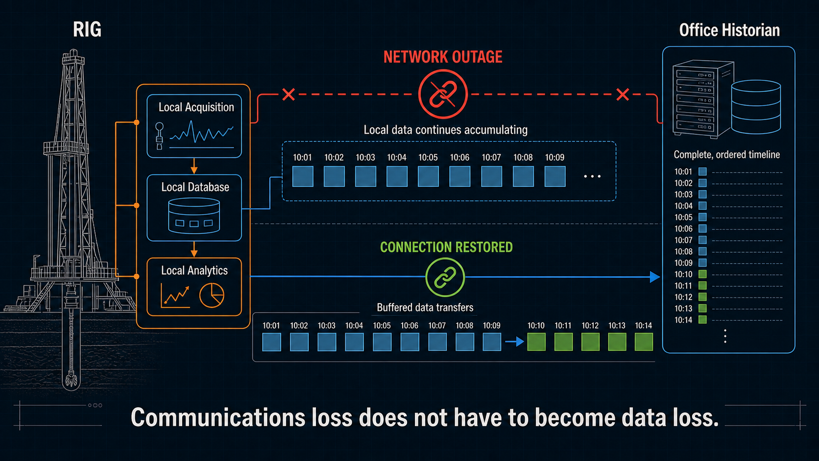
Communications loss does not have to become data loss.

Reconnecting Creates Deduplication Problems

Suppose a rig stores 30 minutes of data locally.

The network returns.

The buffered data is transmitted.

Meanwhile, some recent samples have already reached the office through another path.

The ingestion system now needs to avoid:

• duplicate rows,
• double-counted events,
• out-of-order timestamps.

This is a classic data-engineering problem with very real drilling consequences.

A duplicated connection event can alter:

• ILT statistics,
• stand counts,
• time totals.

A duplicated sensor stream can distort:

• distributions,
• model inputs.

Therefore ingestion should ideally be idempotent:

replaying the same source data should not create a second version of the same observation unless the source itself represents a legitimate revision.

The “Latest Value” Is More Complicated Than It Sounds

Suppose three sources contain mud weight.

Daily report

12.0 ppg

Mud database

12.2 ppg

Manual engineer entry

12.1 ppg

Which is the current value?

The answer cannot be determined from numeric magnitude.

The data architecture needs rules about:

• source authority,
• freshness,
• operational scope.

Different fields may have different authoritative sources.

For example:

• current RPM → rig stream,
• active BHA → validated BHA record,
• formation interpretation → geology source.

A single global rule such as:

newest timestamp wins

can be unsafe.

The Data Model Should Represent the Physical Well

Database convenience should not override drilling reality.

A useful drilling information hierarchy may include:

$$Operator \rightarrow Field \rightarrow Pad \rightarrow Well \rightarrow Wellbore \rightarrow BHA\ Run \rightarrow Interval \rightarrow Event$$

Not every application needs every level.

But ignoring the hierarchy creates ambiguity later.

This becomes especially important when:

• wells are sidetracked,
• multiple plans exist,
• BHAs are rerun,
• historical offsets are compared.

WITS and WITSML Solve Only Part of the Problem

Industry data interfaces are extremely valuable.

They make it possible to exchange rig information without building every connection from scratch.

But a valid data stream still does not automatically answer:

• Is this the correct channel?
• Is the unit correct?
• Is the sensor calibrated?
• Is the timestamp aligned?
• Is the value stale?
• Which wellbore does it belong to?
• Which BHA was active?

SPE-191797 itself describes an operational system that had to consume not just WITS/WITSML but also:

• PLC data,
• OPC-connected sources,
• mudlogger information,
• daily-report context.[1]

The practical conclusion is:

Data transport standards are an important layer of drilling data engineering, not a complete substitute for it.

Real-Time and Historical Analytics Need the Same Definitions

Suppose the real-time system defines rotary drilling one way.

The post-well database uses a different rule.

Now:

real-time rotary ROP

and:

historical rotary ROP

are not directly comparable.

Likewise, if:

• MSE equation changes,
• slide filtering changes,
• connection detection changes,

historical KPIs may drift over time because the software changed—not because drilling performance changed.

A mature analytics platform should therefore version:

• algorithms,
• definitions,
• transformations.

This allows an engineer to distinguish:

operational improvement

from:

methodology change.

Model Version Is Part of the Result

Suppose:

MSE v1

uses surface RPM.

MSE v2

includes motor-adjusted RPM.

The two values may differ materially.

Calling both:

MSE

without preserving the methodology creates ambiguity.

Likewise:

• torque-and-drag model version,
• hydraulics model version,
• data-quality logic version

may matter when comparing results across years.

Derived engineering data should therefore be treated more like calculated laboratory results than casual spreadsheet columns.

A Practical Example: Real-Time Hydraulics

Consider a hydraulic model calculating expected standpipe pressure.

The surface stream provides:

• flow,
• RPM,
• measured SPP.

The contextual layer provides:

• mud properties,
• drillstring geometry,
• BHA,
• bit nozzle area,
• hole/casing geometry.

The state layer provides:

• whether the current operating condition is appropriate for the calculation.

Now imagine five data-engineering failures.

Failure 1 — Wrong units

Flow arrives in a different unit than expected.

Failure 2 — Stale mud properties

The well was weighted up but the contextual record was not updated.

Failure 3 — Previous BHA still active

The model uses the old nozzle configuration.

Failure 4 — Timestamp mismatch

SPP and flow are offset by several seconds during a pump transition.

Failure 5 — Wrong wellbore

A sidetrack is evaluated using the original-well trajectory.

The hydraulic equations can be coded perfectly in every case.

The answer can still be wrong.

That is why data engineering is part of model validity.

A Practical Processing Pipeline

A conceptual real-time drilling pipeline might be:

1. Acquire

Receive data from:

• rig control,
• EDR,
• WITS/WITSML,
• MWD,
• mudlogging,
• reporting systems.

2. Identify

Resolve:

• rig,
• well,
• wellbore,
• source,
• channel.

3. Normalize

Standardize:

• engineering variable name,
• units,
• sign conventions.

4. Synchronize

Align measurements in time with explicit rules for:

• differing frequencies,
• latency,
• stale data.

5. Validate

Detect:

• missing,
• outlier,
• biased,
• frozen,
• questionable values.

6. Attach context

Resolve current:

• BHA,
• surveys,
• casing,
• mud properties,
• formation where available.

7. Establish operational state

Classify the rig activity.

8. Calculate

Run:

• deterministic calculations,
• statistical features,
• event models.

9. Persist

Store:

• measurements,
• context,
• calculated outputs,
• provenance.

10. Deliver

Provide:

• dashboards,
• alerts,
• APIs,
• reports,
• AI access.

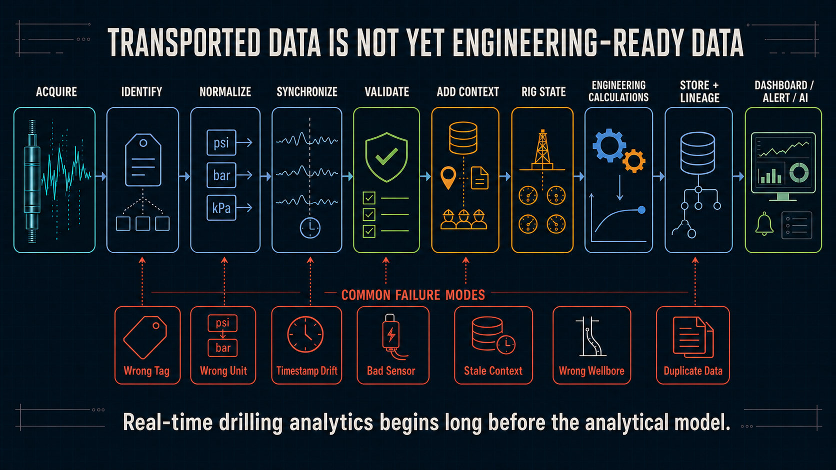
Real-time drilling analytics begins long before the analytical model.

This Work Is Mostly Invisible When It Succeeds

When the data system works correctly, the engineer sees:

• a clean plot,
• the correct BHA,
• the correct formation,
• an accurate model comparison.

Nothing appears remarkable.

When it fails, the symptoms appear elsewhere:

• nonsensical MSE,
• wrong offset,
• false hydraulic alarm,
• duplicate connection,
• incorrect friction factor,
• AI answer citing the wrong wellbore.

Data engineering is therefore unusual.

Success looks like:

nothing went wrong.

That can make the work easy to undervalue.

Drilling Data Engineering Is Part of the Engineering Method

This is the broader conclusion.

Consider a scientific experiment.

No engineer would separate:

instrument calibration

from:

experimental validity.

Drilling analytics should be viewed the same way.

Choices about:

• sensor source,
• unit conversion,
• timestamp alignment,
• context selection,
• depth mapping,
• filtering

directly affect the analytical conclusion.

Therefore these decisions belong in the documented engineering methodology.

They should not remain undocumented implementation details hidden inside software.

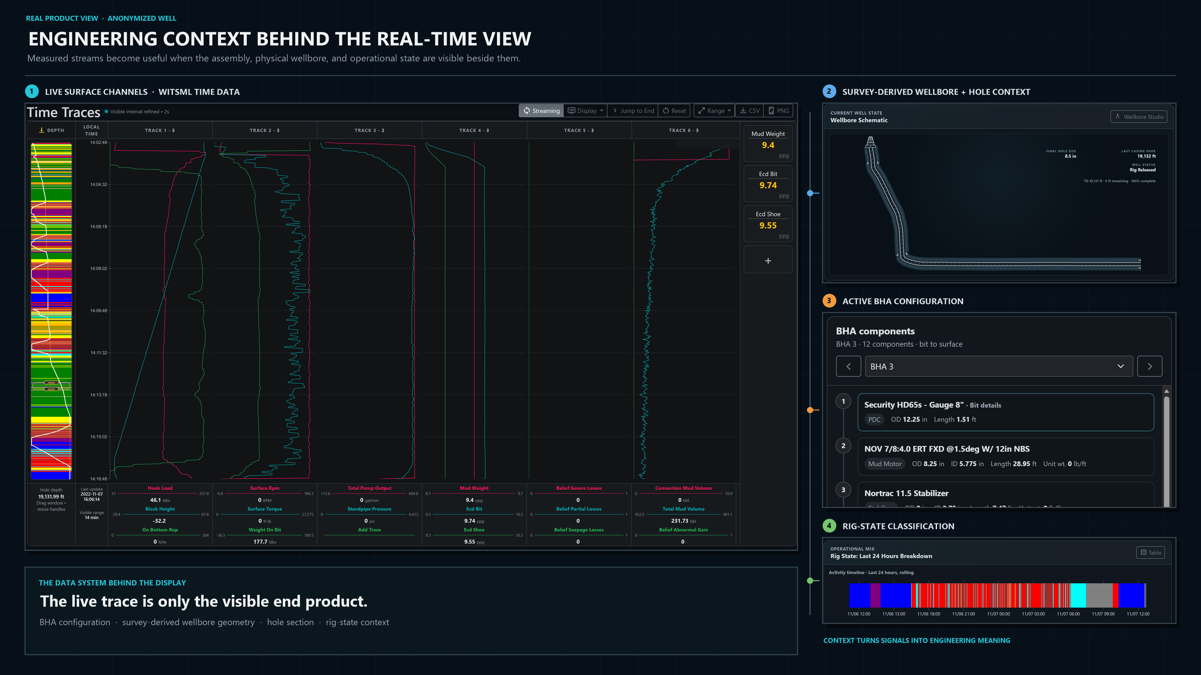
The visible real-time view depends on aligned measurements, active configuration, physical wellbore context, and operational state.

What a Drilling Engineer Should Ask About an Analytics Platform

When evaluating a real-time analytics result, useful questions include:

Where did this measurement come from?

Which rig system or sensor?

What does the channel physically represent?

Surface or downhole? Hole depth or bit depth?

Is the value current?

When was it last updated?

What context was used?

Which:

• BHA,
• mud properties,
• survey,
• wellbore?

Was the sensor quality checked?

Could the model be responding to bad data?

What transformations were applied?

Was the data:

• averaged,
• filtered,
• interpolated?

Can the result be traced back?

Can we recover the evidence behind the KPI?

Those questions are not software trivia.

They determine whether the number deserves engineering trust.

Conclusion

Real-time drilling analytics is often described from the end of the pipeline.

We talk about:

• MSE,
• torque and drag,
• hydraulics,
• dysfunction detection,
• AI.

But those systems depend on a much less visible layer.

Before a model can interpret the well, software has to determine:

• which data belongs to which engineering variable,
• when the measurement occurred,
• whether it is trustworthy,
• what units it uses,
• which wellbore it belongs to,
• which BHA was active,
• what mud and geometry existed at that moment.

Then the system must preserve that information through:

• buffering,
• synchronization,
• storage,
• calculation,
• historical retrieval.

That is data engineering.

And in drilling, it is not merely software plumbing.

It is part of the engineering definition of the problem.

A sophisticated model supplied with incoherent inputs is not sophisticated drilling intelligence.

The real foundation is a data system capable of turning many independent rig and engineering sources into one trustworthy representation of:

what the well was doing, where it was doing it, and under what physical configuration.

Everything else is built on top of that.

---

References

1. Shahri, M., Kutlu, B., Thetford, T., Nelson, B., Wilson, T., Behounek, M., Ambrus, A., and Ashok, P. Adopting Physical Models in Real-Time Drilling Application: Wellbore Hydraulics. SPE-191797-MS, SPE Liquids-Rich Basins Conference—North America, Midland, Texas, 2018.

2. Shahri, M., Wilson, T., Thetford, T., Nelson, B., Behounek, M., Ambrus, A., D'Angelo, J., and Ashok, P. Implementation of a Fully Automated Real-Time Torque and Drag Model for Improving Drilling Performance: Case Study. SPE-191426-MS, SPE Annual Technical Conference and Exhibition, Dallas, Texas, 2018.

3. Behounek, M., Thetford, T., Yang, L., Hofer, E., White, M., Ashok, P., Ambrus, A., and Ramos, D. Human Factors Engineering in the Design and Deployment of a Novel Data Aggregation and Distribution System for Drilling Operations. SPE/IADC-184743-MS, SPE/IADC Drilling Conference and Exhibition, The Hague, Netherlands, 2017.

4. Ashok, P., Ambrus, A., Ramos, D., Lutteringer, J., Behounek, M., Yang, Y. L., Thetford, T., and Weaver, T. A Step by Step Approach to Improving Data Quality in Drilling Operations: Field Trials in North America. SPE-181076-MS, SPE Intelligent Energy International Conference and Exhibition, Aberdeen, Scotland, 2016.

5. Ashok, P., van Oort, E., and Ambrus, A. Automatic Sensor Data Validation: Improving the Quality and Reliability of Rig Data. SPE-163726-MS, SPE Digital Energy Conference and Exhibition, The Woodlands, Texas, 2013.