Depth-Based and Time-Based Analysis of Real-Time Drilling Data

Time preserves operational sequence and transient behavior. Depth preserves location and makes geological and offset comparisons possible. Changing between the two can also change the statistical meaning of the data.

A standpipe-pressure decrease begins at 10:42 AM.

Torque becomes erratic twenty seconds later.

ROP falls after another thirty seconds.

A time-based plot makes that sequence easy to see.

Now suppose the same event occurred at 13,850 ft.

The engineer wants to know:

• whether the same depth was troublesome on an offset,
• whether a formation boundary is nearby,
• whether MSE normally changes there,
• and whether previous BHAs behaved similarly.

For those questions, a depth-based plot is much more useful.

It is the same drilling operation.

It is the same data.

But the two views answer different engineering questions.

That distinction becomes important because most real-time rig measurements are acquired in time, while many drilling decisions and post-well comparisons are made in depth.

Converting between those domains is often treated as a visualization task:

Change the x-axis from time to measured depth.

In reality, more has changed than the axis.

The data is now being organized, weighted, aggregated, and potentially filtered according to a different variable.

The result can alter:

• averages,
• distributions,
• apparent trends,
• visibility of short events,
• and even which observations appear to belong together.

The key principle is therefore:

Time-based and depth-based analysis are complementary representations of drilling data, not interchangeable versions of the same analysis.

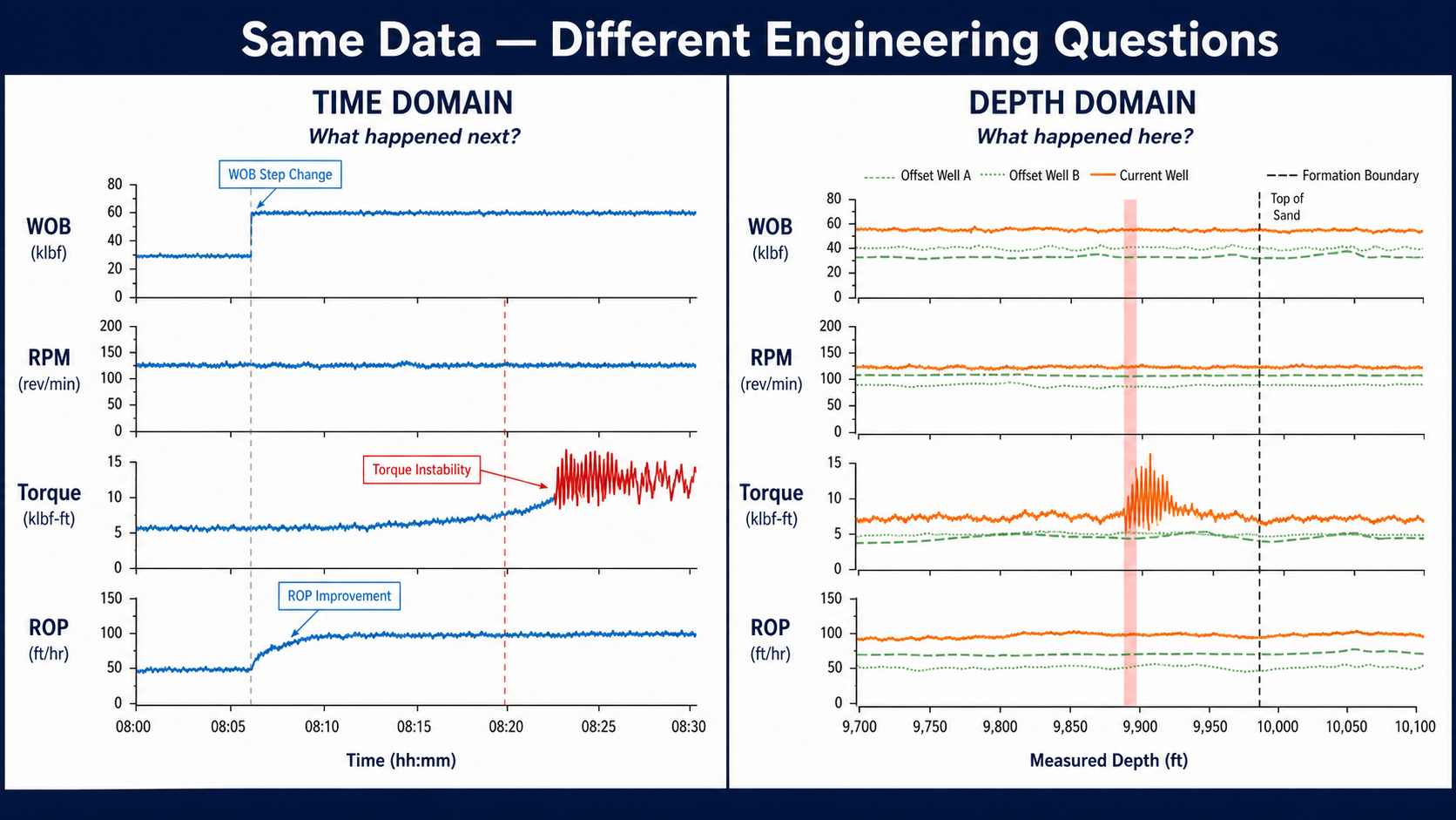
Time preserves operational sequence; depth preserves where the response occurred in the well.

Real-Time Rig Data Naturally Arrives in Time

Most electronic drilling data begins as a time series.

At each timestamp the system may record:

• hole depth,
• bit depth,
• hook load,
• WOB,
• surface RPM,
• torque,
• standpipe pressure,
• pump rate,
• flow out,
• ROP.

A simplified record might look like:

Time	Hole Depth	Bit Depth	WOB	RPM	Torque	SPP
10:00:00	12,500.0	12,500.0	32	120	15,200	4,550
10:00:01	12,500.04	12,500.04	32	120	15,350	4,555
10:00:02	12,500.08	12,500.08	33	120	15,500	4,560

If the acquisition frequency is 1 Hz, each row represents approximately one second.

That has an important statistical consequence:

The sampling system gives equal representation to equal units of time—not equal units of hole drilled.

One second drilling rapidly receives one sample.

One second drilling slowly also receives one sample.

But the footage represented by those samples is different.

That becomes important when the data is later transformed to depth.

Time Is the Natural Domain for Sequence and Causality

Time-based analysis is generally strongest when the engineering question involves:

• what happened first,
• how rapidly something changed,
• whether one signal responded to another,
• how long a condition persisted,
• or how an operation transitioned from one state to another.

Consider a parameter change.

At 14:12:30:

WOB increases from 28 to 36 klbf.

At 14:12:38:

surface torque begins increasing.

At 14:12:45:

ROP improves.

At 14:13:05:

torque starts oscillating severely.

The time domain preserves that sequence.

The engineer can ask:

Did ROP improve immediately after increasing WOB?

Did the torque instability appear before or after the parameter change?

Was the oscillation persistent or just one transient?

These are fundamentally temporal questions.

The exact depth associated with the event is useful context, but depth alone does not describe the sequence as naturally.

Depth Is the Natural Domain for Location

Now consider a different question:

Why does torque increase around 14,000 ft?

The engineer may want to compare the response with:

• formation tops,
• trajectory,
• hole angle,
• tortuosity,
• BHA changes,
• bit-run history,
• offsets.

Those quantities are naturally tied to location in the well.

A depth-based view allows:

Current Well

to be aligned against:

Offset Well A

and:

Offset Well B

at corresponding intervals.

SPE/IADC-184743 describes this exact motivation for depth-based offset overlays: real-time parameters could be plotted against historical wells and adjusted for depth shifts, with formation markers added to assist interpretation.[1]

Depth therefore provides a common coordinate for comparing wells that were drilled:

• on different dates,
• at different ROP,
• by different crews.

Clock time has almost no value for that comparison.

Depth does.

Time and Depth Are Not One-to-One

The most important complication is that time and depth do not have a simple one-to-one relationship.

During rotary drilling:

• time advances,
• hole depth increases,
• bit depth generally increases.

During a connection:

• time advances,
• hole depth stays constant,
• bit depth may change slightly or remain static.

During a trip:

• time advances,
• hole depth stays constant,
• bit depth can move thousands of feet.

During reaming:

• bit depth changes,
• but new hole may not be created.

During circulation off bottom:

• time advances,
• neither hole depth nor bit depth necessarily changes much.

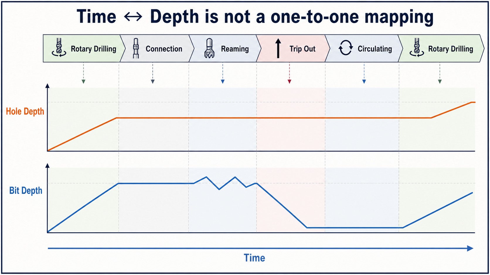
Time continues through drilling, connections, reaming, circulation, and trips while hole depth and bit depth respond differently.

This means there are actually several potential depth axes.

Hole depth

represents the deepest drilled extent of the well.

It is usually the logical coordinate for:

• as-drilled ROP,
• drilling performance,
• formation comparison.

Bit depth

represents where the bit currently is.

It is often more useful for:

• tripping,
• reaming,
• mechanical events,
• torque-and-drag analysis.

TVD

can be useful for vertically referenced geology and pressure relationships.

Formation-relative depth

can be better for comparing equivalent geological intervals between wells.

The correct depth variable depends on the question.

“Plot it by depth” is therefore incomplete unless the type of depth has also been defined.

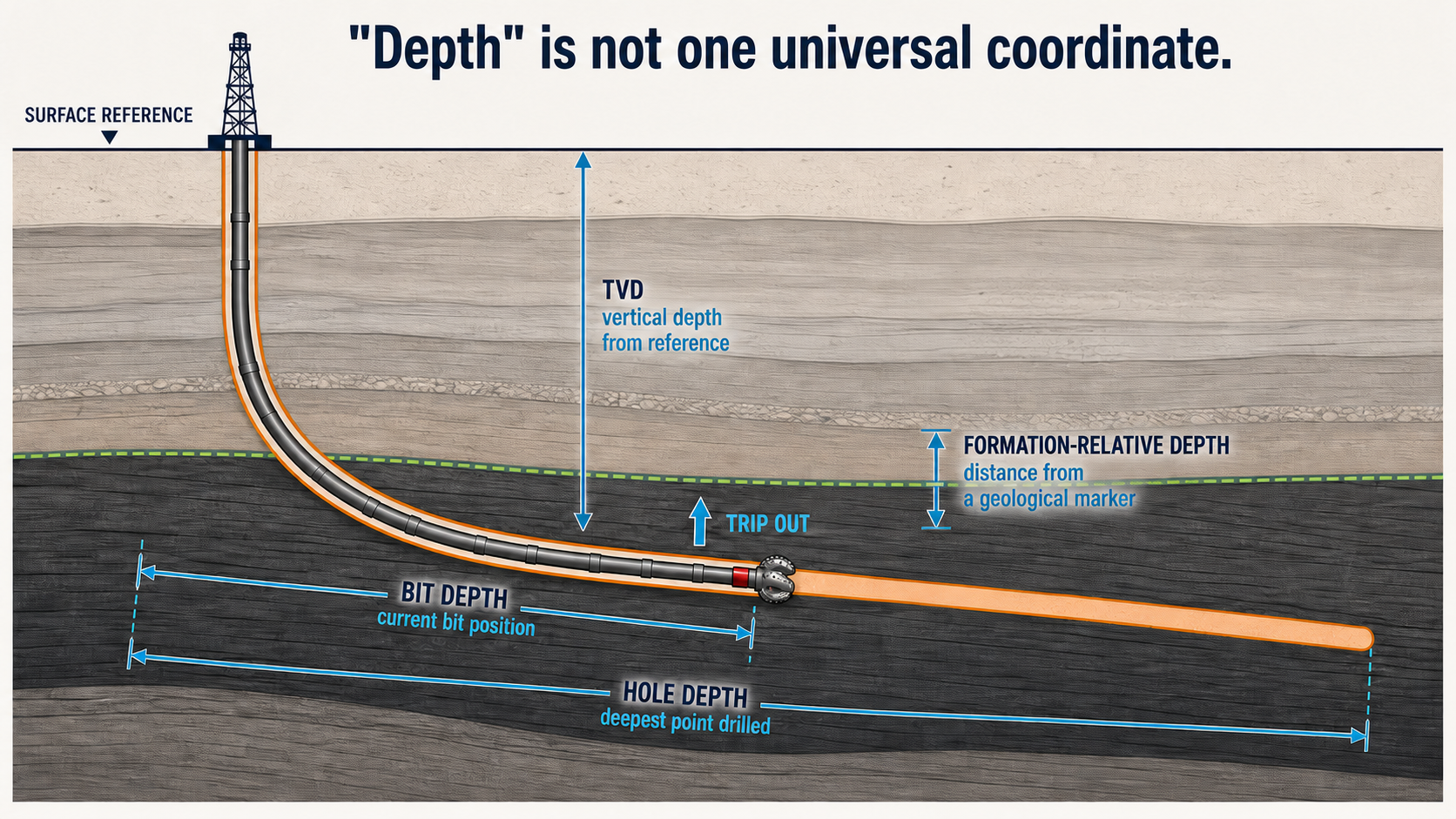
Hole depth, bit depth, TVD, and formation-relative depth are different coordinates suited to different engineering questions.

Rig State Should Usually Be Applied Before Depth Conversion

Suppose all real-time samples are simply grouped by hole depth.

At 14,000 ft the rig spends:

• 15 minutes drilling,
• 5 minutes reaming,
• 4 minutes circulating,
• 6 minutes making a connection.

Every one of those samples may inherit approximately the same hole depth.

If the data is then averaged into a depth bin, the resulting torque, RPM, flow, or WOB values can contain several physically different operations.

The depth bin is numerically valid.

The engineering population is not.

A better sequence is usually:

1. validate the data,
2. identify rig state,
3. select the operational population,
4. then convert or aggregate by depth.

For a drilling-performance analysis:

drilling data → depth

is much more meaningful than:

all time-series data → depth.

This is one reason operational-state classification is such important infrastructure for depth-based analytics.

Faster Drilling Produces Fewer Samples per Foot

This is one of the less obvious consequences of time-based acquisition.

Assume a 1-Hz data stream.

At:

20 ft/hr

the bit advances:

$$\frac{20}{3600} = 0.0056\ ft/sec$$

That produces roughly:

$$180\ samples/ft$$

At:

200 ft/hr

the bit advances:

$$0.0556\ ft/sec$$

or roughly:

$$18\ samples/ft$$

The slow interval produces approximately ten times as many time samples per foot.

Nothing is wrong with the acquisition system.

It is doing exactly what it was designed to do:

sampling uniformly in time.

But if every raw sample is later treated as an equal observation in a depth-oriented analysis, the slower footage receives much greater statistical representation.

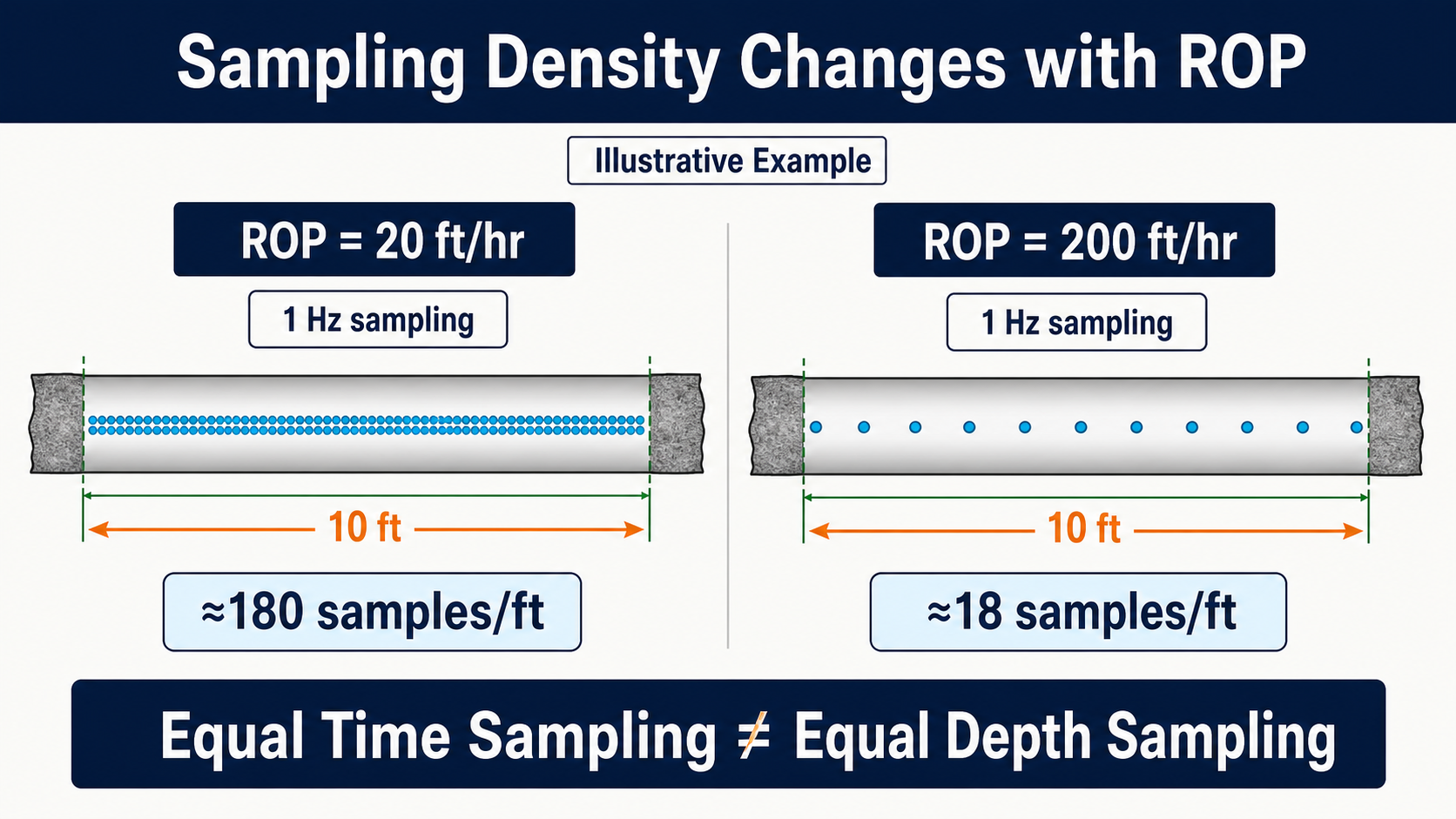
A fixed-frequency time series contains more samples per foot when the bit is drilling slowly.

"Average ROP" Can Mean Different Things

Consider a simple hypothetical section.

The first 100 ft is drilled at:

100 ft/hr

The next 100 ft is drilled at:

200 ft/hr

Total footage:

$$200\ ft$$

Time required:

First interval:

$$100 / 100 = 1.0\ hr$$

Second interval:

$$100 / 200 = 0.5\ hr$$

Total:

$$1.5\ hr$$

The section drilling rate is therefore:

$$ROP_{section} = \frac{200}{1.5} = 133.3\ ft/hr$$

Now calculate an equal-footage average of the two ROP values:

$$\frac{100+200}{2} = 150\ ft/hr$$

Both numbers arise legitimately from the same drilling.

But they answer different questions.

133 ft/hr

answers:

How quickly was the section actually drilled?

It reflects the fact that more time was spent in the slower interval.

150 ft/hr

answers something closer to:

What was the average ROP across equally weighted footage intervals?

The difference is not a mathematical error.

It is a weighting decision.

This is why every drilling-performance KPI should define whether its population is weighted by:

• time,
• footage,
• stands,
• events,
• or another unit.

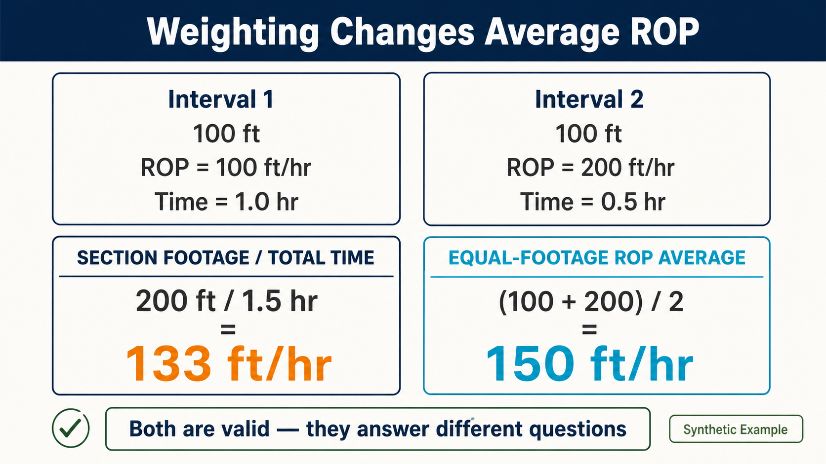
Time-weighted and equal-footage ROP averages can both be valid, but they answer different engineering questions.

Neither Weighting Method Is Universally Better

The correct weighting depends on the engineering question.

If the objective is:

How much rig time did this interval consume?

time weighting is highly relevant.

If the objective is:

How did drilling performance vary through the formation?

equal-depth bins may be more useful.

If the objective is:

How did each stand perform?

stand-level aggregation may be preferable.

SPE-205844 provides a good example of the latter approach. The bit-wear study filtered the surface data to the appropriate rotary drilling population, calculated statistics for individual stands, and plotted median values by measured depth.[3]

That changes millions of individual sensor measurements into a much smaller number of mechanically meaningful observations.

The statistical unit becomes:

stand drilled

rather than:

one second of sensor data.

Depth Binning Is an Analytical Decision

Once drilling data is transformed to depth, another choice appears:

How large should the depth interval be?

Possible intervals might include:

• 1 ft,
• 5 ft,
• 10 ft,
• one stand,
• 100 ft,
• formation interval.

Smaller bins preserve more detail.

Larger bins suppress variability and simplify comparison.

But larger is not always better.

Suppose a dysfunction persists for only 20 ft.

A 100-ft median may almost completely hide it.

Conversely, a 1-ft statistic may be unnecessarily noisy for evaluating the performance of a BHA over several thousand feet.

The correct resolution should match the physical scale of the question.

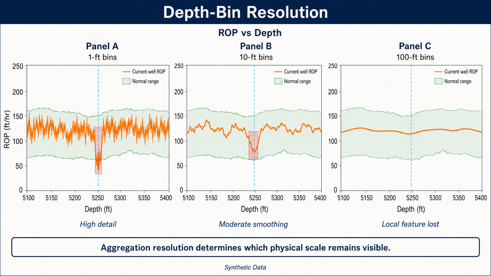
Depth-bin size determines whether a local performance change remains visible or is smoothed into a section-scale trend.

Bit failure

stand-level trends may be appropriate.

Formation benchmarking

tens or hundreds of feet may be appropriate.

Survey response

individual survey intervals may matter.

Short mechanical event

the time domain may be more useful than depth aggregation at all.

Mean, Median, Maximum, and Percentiles Preserve Different Information

Changing to depth does not determine how samples inside each depth bin should be summarized.

Suppose torque within a 10-ft bin contains:

• mostly 14–16 klbf-ft,
• with one brief spike to 30 klbf-ft.

The:

mean

may increase only slightly.

The:

median

may barely change.

The:

maximum

will clearly preserve the spike.

The:

P95

may capture elevated mechanical behavior without being dominated by one sample.

Which statistic is correct?

Again, it depends on the question.

For stable parameter benchmarking:

median may be useful.

For detecting short mechanical extremes:

maximum or upper percentiles may matter more.

For energy calculations:

another aggregation method may be required.

There is no universal depth-aggregation statistic.

Depth Aggregation Can Hide Temporal Events

Imagine a 30-ft interval drilled in ten minutes.

For nine minutes, torque is stable.

For thirty seconds, severe oscillation occurs.

Then drilling stabilizes again.

A depth-based median may make the interval look completely normal.

A time-series view immediately exposes the event.

This does not make depth aggregation bad.

It means the representation has intentionally compressed time-domain information.

That leads to an important practical rule:

Use depth to locate the problem; use time to investigate the event.

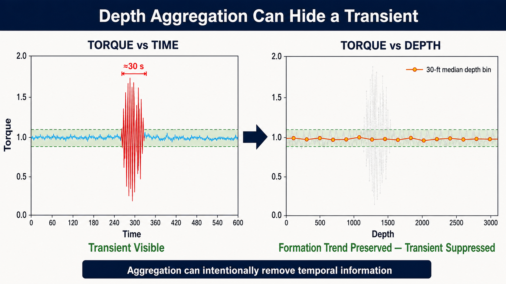
Depth aggregation can summarize formation-scale behavior while hiding short-lived mechanical events.

Time Windows and Depth Windows Also Filter Data Differently

SPE-186166 describes filtering its drilling-efficiency indicator using moving averages defined over either time or depth.[2]

Those approaches can behave differently when ROP changes.

Consider:

Five-minute moving window

At 60 ft/hr, it represents approximately:

5 ft

of hole.

At 240 ft/hr, it represents approximately:

20 ft

of hole.

The temporal smoothing stays constant.

The geological interval does not.

Now consider:

20-ft moving depth window

At 60 ft/hr, it spans approximately:

20 minutes

of drilling.

At 240 ft/hr, it spans:

5 minutes.

The geological scale stays constant.

The temporal scale changes.

This means filter design should also follow the engineering objective.

If investigating:

equipment dynamics

a time window may be more defensible.

If investigating:

formation-related behavior

a depth window may be more defensible.

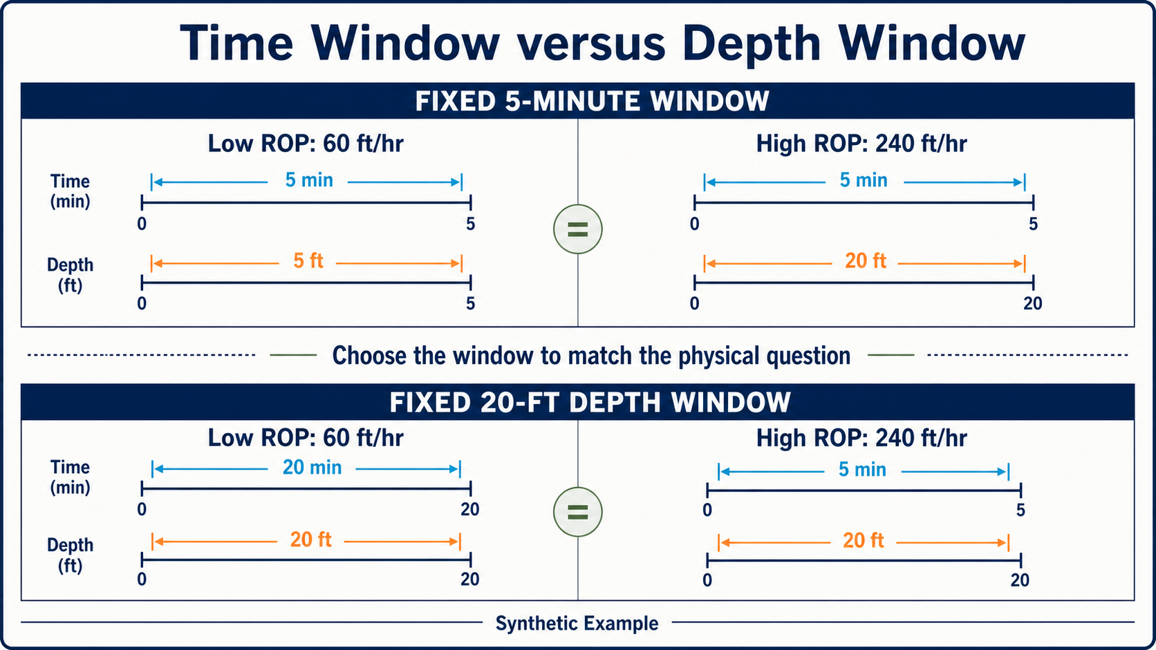
A fixed time window preserves duration but spans variable footage; a fixed depth window preserves footage but spans variable duration.

Time-Based Analysis Is Better for Operational Transitions

Several drilling problems are fundamentally about transitions.

Examples include:

• staging pumps,
• starting rotation,
• tagging bottom,
• changing WOB,
• changing RPM,
• beginning a slide,
• connection sequences.

These operations are naturally described as:

before → during → after.

Time makes those boundaries explicit.

It also allows engineers to measure response lag.

For example:

Parameter change at:

10:15:00

Torque response at:

10:15:04

ROP response at:

10:15:12

That relationship can become difficult to see once the same data is collapsed into depth bins.

Depth-Based Analysis Is Better for Repeated Geological Comparison

Other questions naturally belong in depth.

For example:

Does MSE increase every time we enter this formation?

Does torque rise near the same point on every offset?

Is bit degradation accelerating after a certain footage?

Which BHA produced the smoothest lateral?

Where did the current well begin underperforming the offset envelope?

SPE/IADC-184743 used depth-based historical overlays specifically to make these kinds of current-versus-offset comparisons practical.[1]

The paper also describes a high-resolution days-versus-depth representation that allowed engineers to locate flat portions of the drilling curve that may be obscured by conventional daily reporting.[1]

That illustrates the real advantage of depth:

location becomes the common indexing variable across wells and across time.

The wells do not need to have been drilled on the same day.

They only need a defensible common location basis.

Time Synchronization Comes Before Either Analysis

A drilling dashboard may combine information from:

• rig PLC data,
• EDR/WITS streams,
• MWD,
• mudlogging,
• manually entered mud properties,
• well plans,
• reporting systems.

SPE-191797 describes a real-time system aggregating multiple data streams and contextual sources before feeding engineering models.[4]

Before asking whether the data should be plotted in time or depth, the streams first have to refer to the same operational moment.

A five-second misalignment can be insignificant for a daily report.

It can materially affect an analysis of:

• pump transients,
• torque response,
• short drilling dysfunctions.

Once mismatched streams are mapped to depth, that temporal error can become more difficult to recognize.

The sensible order is:

Synchronize first. Contextualize second. Transform third.

Interpolation Creates New Rows, Not New Measurements

Suppose one dataset contains a drilling value every 10 ft.

Another contains one value every foot.

It is tempting to interpolate the sparse dataset onto the 1-ft grid.

That may be necessary for plotting or numerical comparison.

But the distinction should remain clear:

Interpolated values are estimates between measurements.

They are not additional observations.

This is the same lesson encountered in the survey-resolution article.

Increasing the row count does not increase the measured information content.

Depth transformation should therefore preserve metadata about:

• original source resolution,
• interpolation,
• binning method,
• aggregation method.

A Practical Example

Consider a hypothetical 300-ft lateral interval.

14,000–14,100 ft

ROP:

150 ft/hr

Torque:

stable.

14,100–14,200 ft

ROP rises to:

230 ft/hr

after a parameter change.

Torque remains stable initially.

14,200–14,220 ft

A severe torsional oscillation develops for approximately two minutes.

14,220–14,300 ft

ROP falls to:

175 ft/hr

and torque stabilizes.

What does the time view show?

It can reveal:

1. exactly when WOB/RPM changed,
2. how quickly ROP responded,
3. when torque oscillation began,
4. whether ROP deterioration followed the dysfunction.

What does the depth view show?

It can reveal:

1. where the parameter change occurred,
2. where the dysfunction occurred,
3. whether offsets show similar behavior,
4. whether a geological boundary coincides with the response.

Both are necessary.

Trying to force the entire investigation into one representation loses information.

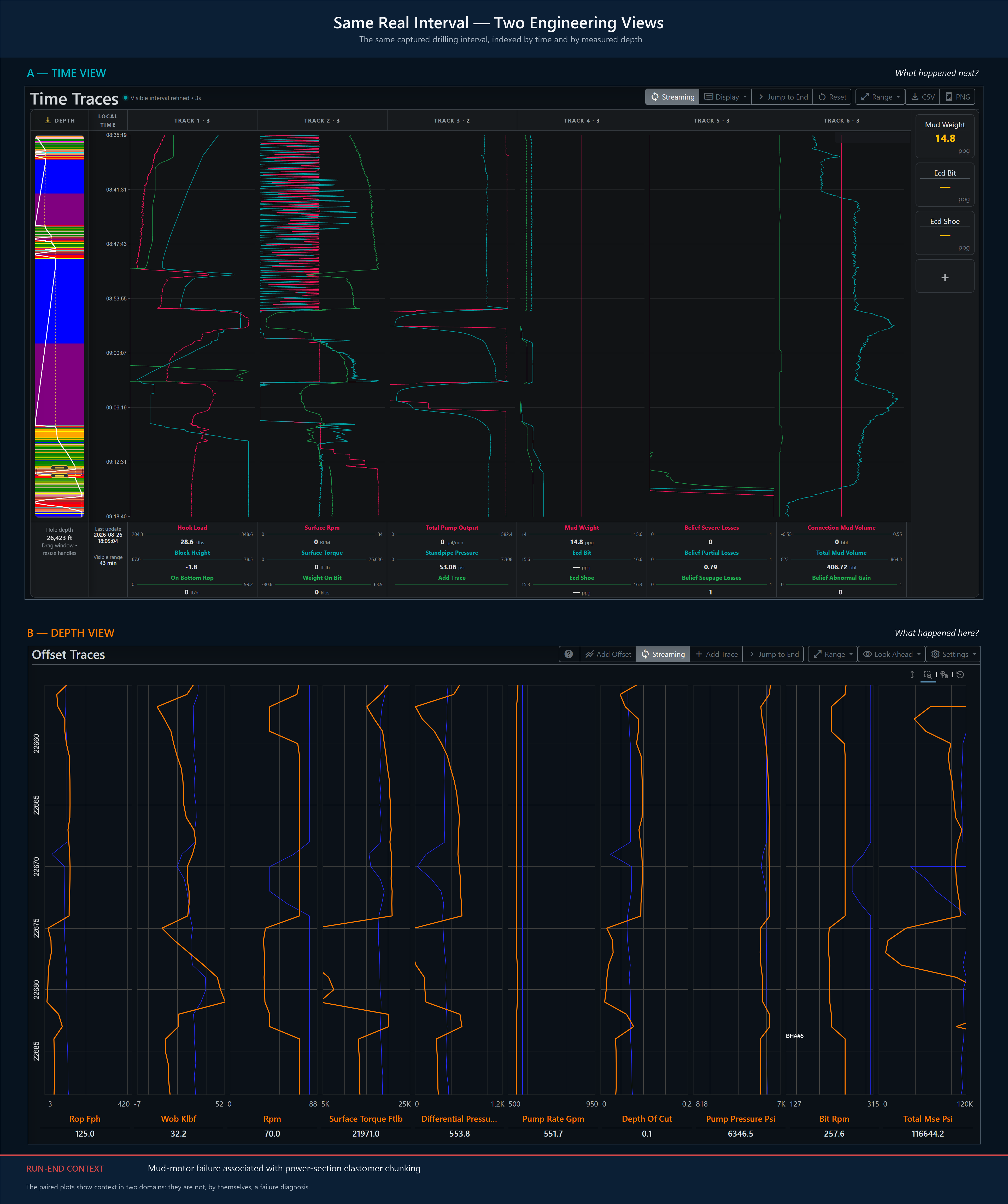
The same drilling interval viewed in time and measured depth. The interval ends at a mud-motor failure associated with power-section elastomer chunking; the plots provide context, not a standalone diagnosis.

A Practical Workflow for Time-to-Depth Transformation

A defensible workflow might look like this.

1. Define the engineering question

Do you need:

• sequence,
• location,
• section performance,
• geological comparison,
• event investigation?

2. Validate and synchronize the source data

Resolve:

• bad sensors,
• missing intervals,
• timestamp problems,
• source latency where known.

3. Classify operational state

Separate:

• drilling,
• sliding,
• reaming,
• tripping,
• connections,
• circulation.

4. Choose the correct depth coordinate

Use:

• hole depth,
• bit depth,
• TVD,
• formation-relative depth

according to the question.

5. Choose the analytical unit

Examples:

• raw sample,
• foot,
• 10-ft interval,
• stand,
• formation.

6. Choose the aggregation statistic

Examples:

• median,
• mean,
• maximum,
• P10/P90.

7. Preserve provenance

Record:

• source frequency,
• state filter,
• depth basis,
• bin size,
• aggregation method,
• interpolation.

8. Retain the time-series source

A depth-derived KPI should be traceable back to the underlying time interval when investigation is required.

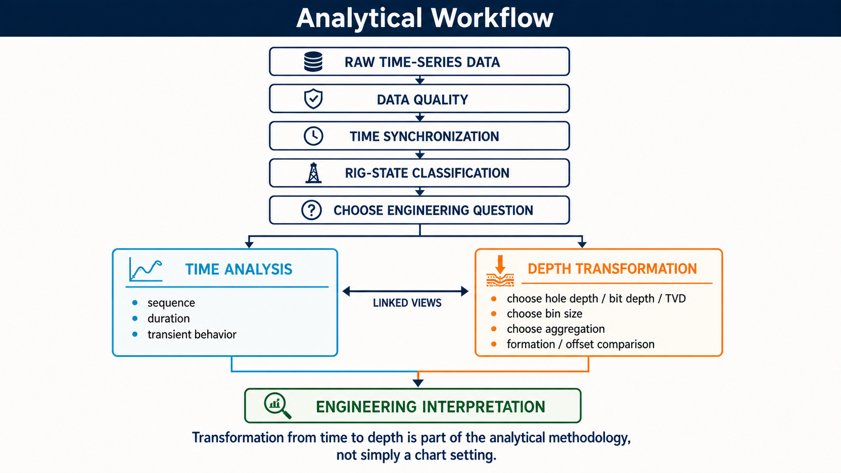
A defensible transformation synchronizes and classifies time-series data before choosing the depth coordinate, binning, and aggregation.

Depth and Time Should Be Linked, Not Compete

The best analytical system should not force the engineer to choose permanently between the two.

A depth anomaly should be clickable back into its underlying time sequence.

A time event should be locatable immediately in the well.

This creates a bidirectional relationship:

$$Time \leftrightarrow Depth$$

For example:

An engineer sees:

MSE increase around 13,600 ft

in a depth-based offset comparison.

They select that interval.

The application opens the corresponding time window.

Now they can inspect:

• parameter changes,
• torque response,
• pump changes,
• rig state,
• transient behavior.

This is far more powerful than maintaining disconnected time and depth reports.

The Axis Is Part of the Model

It is easy to treat the x-axis as presentation.

But in drilling analytics, the x-axis determines:

• how observations are grouped,
• how observations are weighted,
• what counts as nearby,
• which features remain visible,
• which comparisons are physically meaningful.

Time asks:

What happened next?

Depth asks:

What happened here?

A stand asks:

What happened during this repeatable drilling unit?

A formation-relative coordinate asks:

What happened at the equivalent geology?

Each representation imposes structure on the same raw measurements.

That structure is part of the analysis.

The Best Answer Often Uses Both

Many drilling investigations naturally follow this sequence:

Depth first

Identify:

• where performance changed,
• where the current well departed from offsets,
• where a mechanical problem repeatedly appears.

Time second

Investigate:

• what preceded the change,
• what the driller changed,
• which signals responded,
• how long the behavior persisted.

Or the reverse:

Time first

A surveillance alert identifies an abnormal event.

Depth second

The engineer determines:

• where it occurred,
• whether the interval is geologically significant,
• whether offsets had the same problem.

Neither domain contains the entire story.

Real-time drilling analysis becomes stronger when the two remain connected.

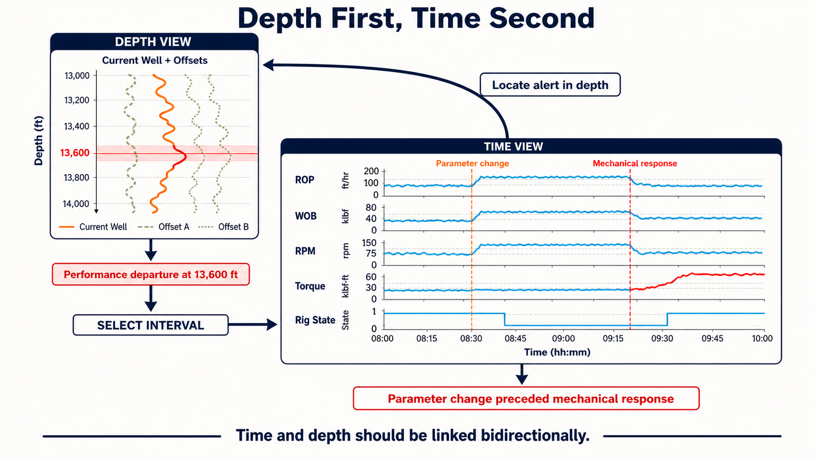
Use depth to locate the interval and time to investigate the operational sequence; alerts should navigate in both directions.

Conclusion

Real-time drilling data begins in time.

Much of drilling engineering ultimately reasons in depth.

The transformation between those domains is useful—but it is not neutral.

Changing from time to depth can alter:

• sample density,
• statistical weighting,
• operational populations,
• event visibility,
• filter behavior.

That means a technically mature drilling analytics workflow should always know:

Which domain is being used?

Why is it appropriate for this question?

How was the transformation performed?

What information may have been lost in the process?

The most useful approach is not to choose between time and depth.

It is to preserve both and use each for the question it answers best.

Time explains how the operation evolved. Depth explains where that behavior belongs in the well.

---

References

1. Behounek, M., Thetford, T., Yang, L., Hofer, E., White, M., Ashok, P., Ambrus, A., and Ramos, D. Human Factors Engineering in the Design and Deployment of a Novel Data Aggregation and Distribution System for Drilling Operations. SPE/IADC-184743-MS, SPE/IADC Drilling Conference and Exhibition, The Hague, Netherlands, 2017.

2. Ambrus, A., Ashok, P., Chintapalli, A., Ramos, D., Behounek, M., Thetford, T. S., and Nelson, B. A Novel Probabilistic Rig Based Drilling Optimization Index to Improve Drilling Performance. SPE-186166-MS, SPE Offshore Europe Conference & Exhibition, Aberdeen, United Kingdom, 2017.

3. Witt-Doerring, Y., Pastusek, P. P., Ashok, P., and van Oort, E. Quantifying PDC Bit Wear in Real-Time and Establishing an Effective Bit Pull Criterion Using Surface Sensors. SPE-205844-MS, SPE Annual Technical Conference and Exhibition, 2021.

4. Shahri, M., Kutlu, B., Thetford, T., Nelson, B., Wilson, T., Behounek, M., Ambrus, A., and Ashok, P. Adopting Physical Models in Real-Time Drilling Application: Wellbore Hydraulics. SPE-191797-MS, SPE Liquids-Rich Basins Conference—North America, Midland, Texas, 2018.