Choosing the Right Sampling Rate for Real-Time Drilling Analytics

High-frequency data can preserve short mechanical events that slower streams or aggressive averaging may hide. For many drilling questions, however, one-second, stand-level, or even longer-horizon summaries are more useful than storing and analyzing every available sample.

A drilling rig can generate data at very different timescales.

Some measurements may update many times per second:

• hook load,
• torque,
• RPM,
• standpipe pressure,
• block position.

Other information may update every few seconds.

Some contextual information may change only once per:

• stand,
• survey,
• BHA run,
• mud check,
• tour.

Now consider three engineering questions.

Question 1

Did hook load spike while pulling through a tight interval?

The relevant behavior might last only a few seconds.

Question 2

Is drilling efficiency deteriorating across the last several stands?

The relevant behavior may develop over hundreds of feet.

Question 3

Is the current BHA drilling this formation more efficiently than the previous BHA?

The relevant scale may be thousands of feet.

All three questions use drilling data.

They should not necessarily use the same sampling rate or aggregation method.

This distinction becomes increasingly important as rigs make higher-frequency data available directly from control systems.

SPE-191426 describes a real-time drilling platform that received high-speed rig-control data commonly at approximately 10 Hz while also integrating slower EDR and contextual information.[1]

That sounds like an argument for using the highest frequency everywhere.

It is not.

The same paper provides an excellent counterexample.

During development of a real-time torque-and-drag workflow, hook-load values were averaged by depth to simplify the data. The resulting dataset looked cleaner—but the averaging reduced the apparent magnitude of genuine overpull events. Eventually the averaging was removed for that part of the analysis so the full overpull could be preserved.[1]

In another drilling application, SPE-205844 began with 1-Hz EDR data and intentionally reduced it to stand-level median values because the objective was to identify longer-term PDC bit-wear trends rather than second-by-second mechanical behavior.[2]

Both approaches were reasonable.

The difference was the engineering question.

The central principle is therefore:

Sampling resolution should be selected from the timescale of the physical behavior being studied—not simply from the maximum frequency the rig can provide.

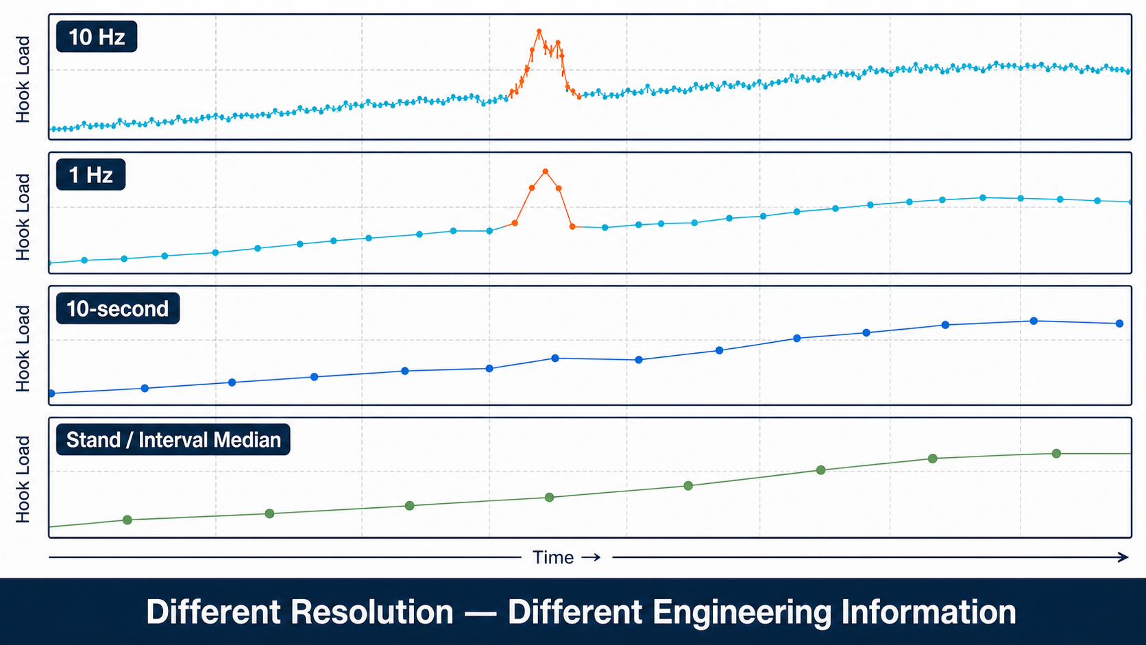
The same signal carries different engineering information at different resolutions.

What Does “High Frequency” Mean on a Drilling Rig?

The phrase can be misleading.

In some drilling-data environments:

10 Hz

may be considered high-frequency data because traditional operational streams may be available at roughly one sample per second or slower.

But 10 Hz should not be interpreted as some universal definition of high frequency.

The useful distinction is relative.

For operational surface data, we might think conceptually in terms of:

Low-frequency contextual data

Examples:

• mud properties,
• BHA configuration,
• casing depth,
• formation tops.

These may change infrequently.

Conventional real-time operational data

Examples:

• WOB,
• torque,
• RPM,
• SPP,
• block position,

sampled perhaps every several seconds or around once per second depending on the system.

Higher-frequency surface data

Rig-control data may be available several times per second.

The engineering question is not:

Is this dataset technically high frequency?

It is:

Is the sampling interval short enough to represent the physical behavior I need to observe?

Sampling Rate Defines What Can Be Seen

Consider a hypothetical hook-load event lasting:

3 seconds.

Sampling every 10 seconds

There may be:

zero samples

inside the event.

Whether the event appears at all depends on the timing of the samples.

Sampling at 1 Hz

Approximately:

3 observations

may represent the event.

Sampling at 10 Hz

Approximately:

30 observations

may represent it.

Nothing about the physical event changed.

Only the observation system changed.

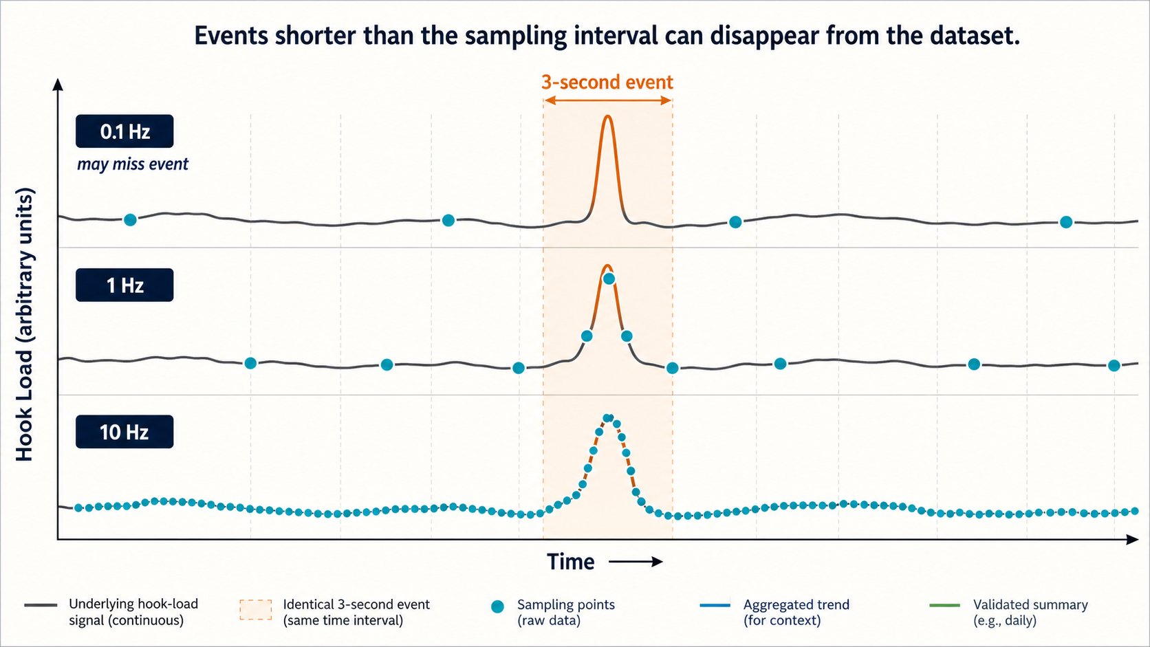
Events shorter than the sampling interval may never enter the stored dataset.

Once Information Is Lost, Interpolation Cannot Recover It

Suppose a 10-Hz signal is reduced to one sample every ten seconds.

Later an analyst wants to investigate a two-second torque disturbance.

They can interpolate between the stored points.

That creates more rows.

It does not recreate the missing torque disturbance.

This is the same information-resolution issue encountered with directional surveys.

Interpolation creates an estimate between measurements.

It does not recreate measurements that were never retained.

That makes raw-data retention valuable when the future analytical questions are not yet known.

Higher Frequency Is Most Valuable for Short Events

Examples of potentially short-lived behavior include:

• overpull,
• transient hook-load excursions,
• rapid torque changes,
• pump transients,
• operational-state transitions.

SPE-191426 provides a particularly useful field example.

The authors compared filtered/averaged tripping data with unfiltered 1-Hz hook-load measurements.

The raw data contained more noise.

It also preserved significant overpulls that the averaging procedure either reduced or failed to represent fully.[1]

After several iterations, the averaging was removed for the relevant analysis.

The important lesson was not:

never average hook load.

It was:

do not average away the physical behavior you are trying to detect.

Noise Reduction and Event Preservation Are Competing Objectives

Consider a signal:

$$x(t) = signal(t) + noise(t)$$

Averaging can suppress noise.

That is useful.

But averaging also suppresses rapid changes in the signal itself.

If the desired information is a slow trend, that is usually acceptable.

If the desired information is the rapid change, it is destructive.

This is why the correct filter depends on the question.

Long-term friction trend

Some smoothing may be highly useful.

Maximum overpull

Averaging can materially understate the value.

Formation-scale MSE trend

Depth aggregation may clarify the pattern.

Short torsional disturbance

The same aggregation may remove it.

The objective should define the filtering—not the desire for a visually smooth trace.

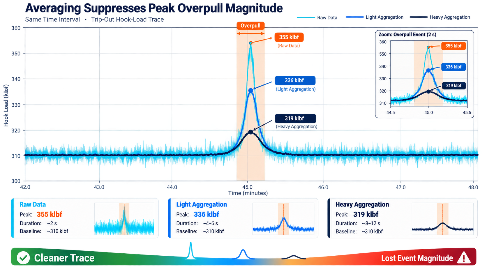
Aggregation can clean a trace while materially understating a short overpull.

High-Frequency Data Does Not Automatically Mean High-Quality Data

Suppose a torque sensor has a:

2,000 ft-lbf bias.

Sampling it at:

0.1 Hz

produces occasional biased readings.

Sampling it at:

10 Hz

produces many more biased readings.

The increased frequency did not improve the measurement.

It only increased the number of observations of the wrong value.

That means:

$$Data\ Value \neq Sampling\ Rate$$

A useful drilling dataset needs both:

• sufficient temporal resolution,
• trustworthy sensor quality.

SPE-181076 emphasizes that poor sensor quality materially limits drilling analytics and can force engineers to clean historical datasets before useful analysis can begin.[3]

More samples cannot compensate for a poorly calibrated sensor.

More Frequency Also Increases the Cost of Bad Data

Consider 20 channels.

At:

0.1 Hz

the dataset contains approximately:

$$20 \times 0.1 \times 86,400 = 172,800$$

channel values per day.

At:

1 Hz

it becomes:

$$1,728,000$$

values per day.

At:

10 Hz

it becomes:

$$17,280,000$$

values per day.

Those are simplified counts, but they illustrate the scaling.

Increasing from 1 Hz to 10 Hz multiplies the raw observation count by ten.

That affects:

• storage,
• transfer,
• database indexing,
• preprocessing,
• synchronization,
• visualization.

The extra data is worthwhile only when it preserves information relevant to a useful engineering application.

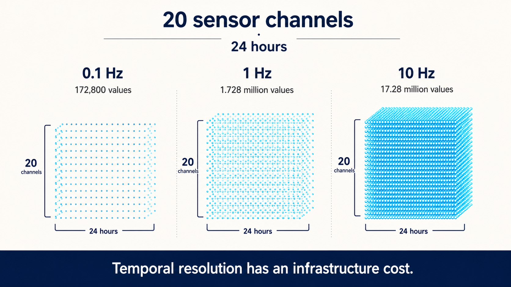
Higher temporal resolution increases raw observations—and infrastructure cost—linearly.

Not Every Channel Needs the Same Sampling Rate

Consider mud weight.

Does an engineer need:

10 mud-weight measurements per second?

Usually the physical property does not change at that timescale.

Now consider hook load during a mechanical event.

Ten observations per second may contain materially more information than one observation every ten seconds.

Therefore a mature data architecture should not assume:

$$Frequency_{all\ channels} = constant$$

Different information classes naturally operate at different timescales.

This is exactly why real-time drilling systems have to merge data of different frequencies.

SPE-191797 describes an architecture combining multiple real-time streams, contextual information, PLC data, WITS data, WITSML, mudlogging, and other sources inside one aggregation layer.[4]

The challenge is not to force them all to become identical.

The challenge is to synchronize them sufficiently for the engineering application.

Time Synchronization Becomes More Important as Frequency Increases

Suppose two sensors are sampled at 10 Hz.

But one stream is delayed by:

2 seconds.

That corresponds to approximately:

20 samples

of temporal offset.

Now imagine investigating whether:

• torque changed before pressure,
• pressure changed before flow,
• WOB changed before ROP.

The event sequence can become incorrect.

At higher sampling frequencies, timestamp quality and synchronization therefore become increasingly important.

More temporal resolution is useful only if the channels are actually aligned in time.

Acquisition Frequency and Analytical Frequency Are Different

This is perhaps the most important architectural distinction.

Suppose the rig provides torque at:

10 Hz.

Does every analytical model need to run at 10 Hz?

No.

We can separate:

Acquisition frequency

How often the original data is captured.

Analytical frequency

How often a particular KPI or model needs to be evaluated.

Display frequency

How often the user interface needs to redraw.

Those three rates can be very different.

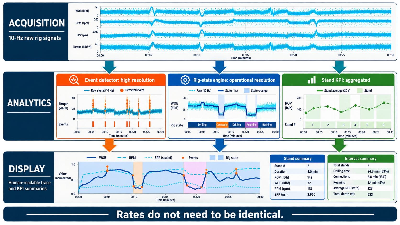
Acquisition, analytical, and display rates do not need to be identical.

The Dashboard Does Not Need Every Raw Point

Suppose a web dashboard displays a six-hour torque trace.

At 10 Hz, that represents:

$$6 \times 3600 \times 10 = 216,000$$

points for one channel.

A monitor may only contain:

1,500 horizontal pixels.

Plotting every raw point does not magically create 216,000 distinguishable visual positions.

A visualization layer can often downsample the display while preserving:

• raw data in storage,
• event detection at higher resolution.

This is a critical architectural principle:

Do not confuse display decimation with analytical data loss.

The engineer does not need to visually render every sample for the system to retain and analyze them.

Raw Data and Derived Data Serve Different Purposes

A useful real-time architecture may retain several levels.

Raw layer

Highest useful acquired resolution.

Purpose:

• event investigation,
• algorithm development,
• forensic lookback.

Operational layer

Cleaned and synchronized data.

Purpose:

• real-time calculations,
• rig state,
• surveillance.

Aggregated layer

Examples:

• stand medians,
• depth bins,
• event summaries.

Purpose:

• performance benchmarking,
• reporting,
• fleet analytics.

These layers are complementary.

The mistake is assuming one representation should replace all the others.

Stand-Level Data Can Be More Useful Than 1-Hz Data

The PDC bit-wear study in SPE-205844 is an excellent example.

The source data was:

1-Hz EDR data.

The researchers:

1. filtered to rotary-on-bottom drilling,
2. identified individual stands,
3. calculated statistics within each stand,
4. used the median wear indicator by measured depth.

Why discard second-by-second detail?

Because the engineering target was:

long-term bit-wear progression.

Local noise and rock variation could obscure the trend.

Stand-level medians made the long-term signal easier to see.[2]

This is not data degradation.

It is purposeful analytical compression.

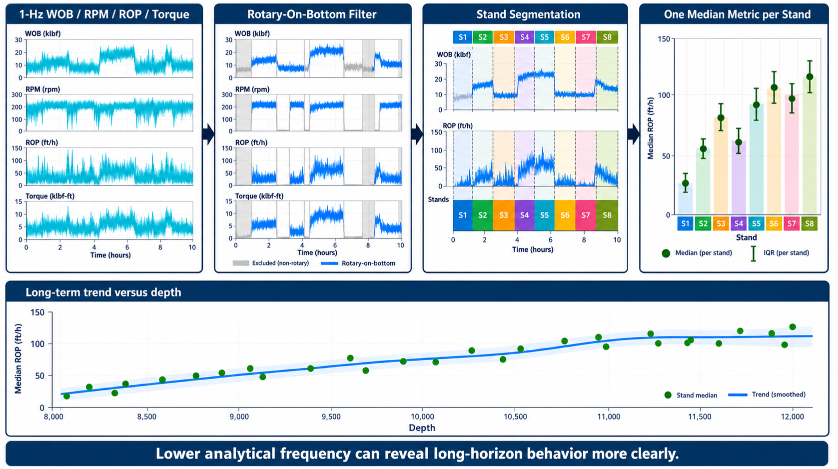
Purposeful aggregation can reveal long-horizon bit-performance behavior more clearly.

Different Failure Modes Have Different Timescales

Hydraulic surveillance provides another useful example.

A circulating-system failure can develop:

• rapidly,
• gradually.

IADC/SPE-189700 analyzed pressure behavior on multiple timescales.

Slow changes in hydraulic behavior were tracked over longer windows, while more sudden pressure behavior was evaluated over a much shorter window.[5]

That illustrates a powerful principle:

one event-detection problem can require multiple analytical timescales simultaneously.

A useful architecture may therefore run:

• short-window detectors,
• medium-window trends,
• long-horizon state estimates

on the same underlying data.

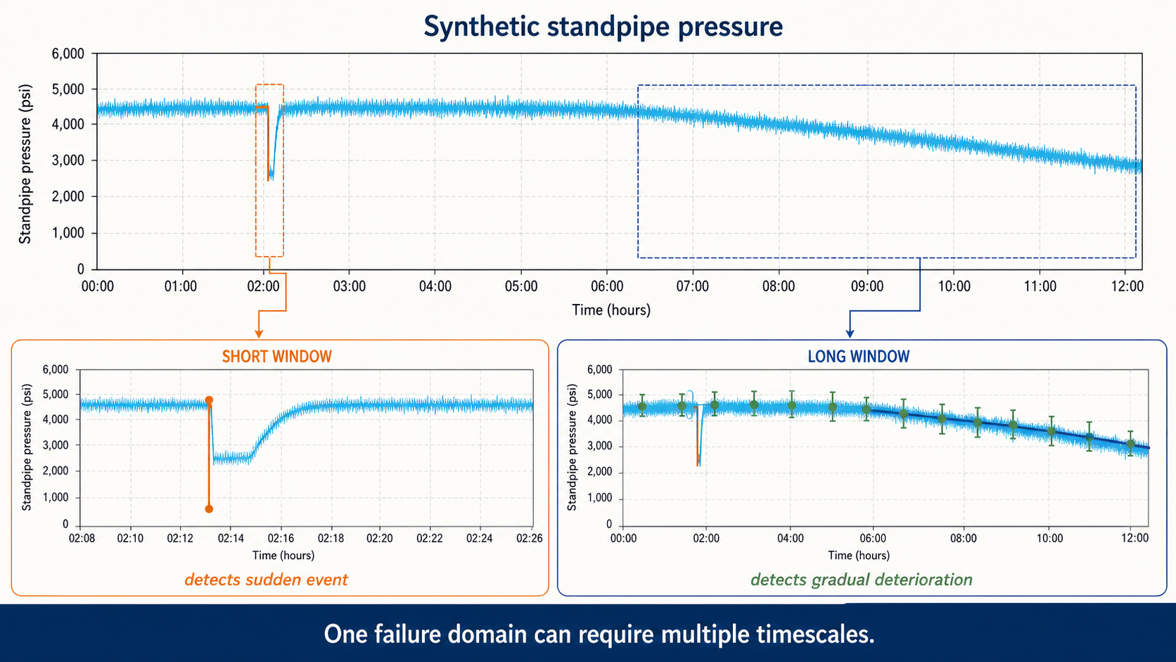
Short windows preserve sudden pressure behavior; long windows reveal gradual deterioration.

One Sampling Frequency Does Not Equal One Timescale

Suppose the stored data is 1 Hz.

We can still calculate:

5-second behavior

using five samples.

2-minute trend

using 120 samples.

30-minute trend

using 1,800 samples.

Stand-level summary

using all samples associated with the stand.

The source sampling rate sets the maximum retained temporal detail.

It does not force every analysis to operate on the same window.

That distinction is fundamental.

Preserve High Resolution, Then Aggregate Intentionally

Once a dataset has been permanently averaged, the original detail is gone.

Therefore, when storage and infrastructure permit, a robust principle is:

retain the highest useful raw resolution and create lower-resolution analytical products from it.

That supports:

• real-time event detection,
• post-event investigation,
• performance reporting,
• future algorithms not yet designed.

But the phrase:

highest useful

matters.

There is no value in retaining meaningless noise at arbitrary frequency simply because the acquisition hardware can produce it.

Downsampling Should Preserve the Statistic You Care About

Suppose we reduce 10-Hz hook-load data to one value per second.

What should that value be?

Possibilities include:

Mean

Good for general level.

Median

Robust to isolated extremes.

Maximum

Useful if peak overpull matters.

Minimum

Useful for certain set-down events.

Range

Useful for variability.

Different aggregation functions preserve different properties.

For an overpull analysis, using only the mean may suppress precisely the quantity of interest.

For long-term trend analysis, maximum values may exaggerate isolated spikes.

Therefore downsampling involves two decisions:

1. time interval,
2. statistic retained.

Min/Max Envelopes Can Preserve Transients in Displays

One practical visualization technique is to preserve both:

• minimum,
• maximum

within each displayed interval.

Suppose 100 raw torque samples must be represented by one screen pixel.

A mean displays only the central tendency.

A min/max envelope can preserve the fact that substantial oscillation occurred inside that interval.

This is especially useful for visualizing high-resolution data over long time windows without rendering every sample individually.

High Frequency Can Expose State Transitions More Clearly

Rig-state classification often depends on changes in:

• block movement,
• pump state,
• rotation,
• bit depth.

Slowly sampled data can blur the transition.

For example:

Rotary drilling stops.

The block moves.

Slips are set.

A connection begins.

At low frequency, several of these transitions may collapse into one observation interval.

Higher-frequency data can help preserve the sequence.

But once the connection is confidently identified, the performance metric may only need:

one connection duration.

Again:

high-frequency input,

low-frequency output.

Event Detection and Continuous Optimization Are Different Problems

This distinction matters.

Event detection

Examples:

• pressure drop,
• overpull,
• short torque disturbance.

Often benefits from preserving faster dynamics.

Continuous performance optimization

Examples:

• MSE trend,
• offset benchmarking,
• bit-wear progression.

Often benefits from:

• smoothing,
• depth aggregation,
• stand statistics.

Trying to feed both problems the same preprocessed dataset can weaken one of them.

A better architecture branches the data according to use case.

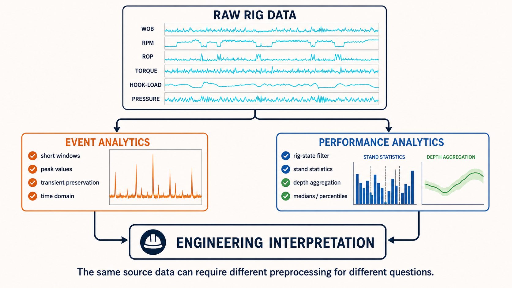
The same source data may need different preprocessing for different engineering questions.

High Frequency Does Not Replace Context

Suppose we sample torque at:

100 times per second.

But we do not know:

• whether the bit is on bottom,
• whether the rig is reaming,
• which BHA is in hole,
• current formation.

The data is temporally detailed.

Its engineering interpretation remains weak.

Conversely, one-second data with strong:

• rig-state,
• BHA,
• formation,
• depth

context may support excellent analysis.

Therefore:

$$Analytical\ Value \neq Frequency\ Alone$$

Useful drilling intelligence requires:

$$Resolution + Quality + Context$$

Higher Frequency Can Magnify Synchronization Problems

Imagine:

• torque at 10 Hz,
• RPM at 1 Hz,
• ROP at 0.1 Hz,
• mud properties updated hours apart.

There is no single natural row where all four quantities were measured simultaneously.

A data system must make decisions about:

• timestamp alignment,
• forward filling,
• interpolation,
• aggregation.

Those decisions become part of the analytical methodology.

This is the hidden data-engineering work behind seemingly simple real-time calculations.

Do Not Forward-Fill Physical Measurements Blindly

Suppose flow updates every second.

One sample is missing.

Forward filling briefly may be harmless for some displays.

Now suppose the stream stops for:

30 seconds

while the software continues repeating the last known value.

The resulting dataset appears complete.

It is not.

A mature system should preserve:

• value,
• timestamp,
• age,
• quality.

A stale value is different from a newly measured value that happens to be identical.

Data Freshness Is Part of Frequency

This leads to an important distinction.

Sampling frequency describes how often the source should update.

Freshness describes how long it has been since it actually updated.

A nominal:

10-Hz channel

that has not changed in five seconds may be experiencing:

• communications loss,
• frozen sensor,
• actual constant process.

The analytics needs enough metadata to tell those situations apart.

Compression Should Be Reversible Where Investigation Matters

Not mathematically reversible.

Operationally traceable.

Suppose a stand-level metric looks abnormal.

The engineer should be able to navigate from:

Stand 214 median MSE

back to:

• the corresponding time interval,
• original torque,
• WOB,
• RPM,
• ROP.

This creates an analytical hierarchy:

$$Summary \rightarrow Interval \rightarrow Raw\ Evidence$$

The summary identifies where to investigate.

The raw data explains what happened.

A Practical Example: An Overpull

Consider a hypothetical trip-out interval.

Normal hook load:

310 klbf

A tight spot produces:

355 klbf

for approximately:

2 seconds.

Then hook load returns toward normal.

Ten-second average

The event may appear only as:

319 klbf

depending on its position in the averaging interval.

The true 45-klbf overpull has been reduced to a 9-klbf increase in the displayed statistic.

One-second data

The event is clearly visible.

Stand/trip summary

The summary could preserve:

Maximum overpull = 45 klbf

without storing every sample in the final report.

The important design lesson is:

summary statistics can preserve the operationally important feature if they are selected intentionally.

A Practical Example: Bit Wear

Now consider a bit run lasting:

50 hours.

Second-by-second MSE or wear indicators fluctuate due to:

• formation variation,
• parameter changes,
• measurement noise.

The question is:

Is bit performance progressively deteriorating over several stands?

High-resolution traces may make that trend harder to see.

Stand-level medians can make it clearer.

Same data infrastructure.

Different analytical scale.

A Practical Multi-Scale Architecture

A mature drilling-data system might conceptually contain four paths.

Level 1 — Raw

Highest useful available frequency.

Retained for:

• forensic review,
• transient algorithms.

Level 2 — Real-Time Operational

Synchronized and quality checked.

Used for:

• rig state,
• engineering calculations,
• alerts.

Level 3 — Event / Stand

Examples:

• connection event,
• overpull event,
• stand statistics.

Used for:

• workflow analytics,
• drilling performance.

Level 4 — Depth / Well / Fleet

Examples:

• 10-ft bins,
• stand medians,
• formation statistics,
• well KPIs.

Used for:

• offsets,
• benchmarking,
• management reporting.

No one level is universally better.

Each answers a different question.

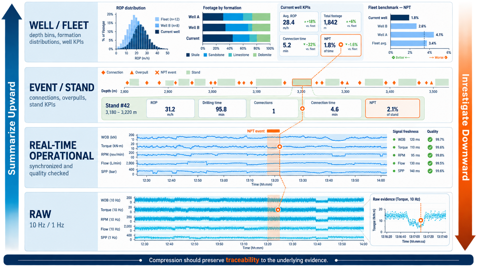
Compression remains useful when summaries stay traceable to the underlying evidence.

How Should the Sampling Rate Be Chosen?

A practical decision process can begin with five questions.

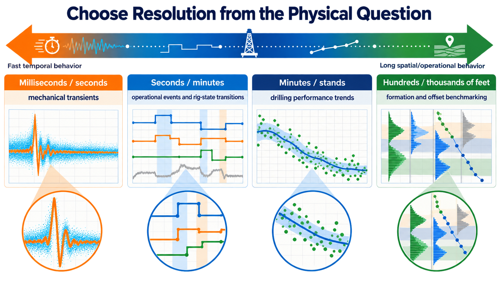
Choose resolution from the physical question rather than prescribing one universal frequency.

1. What physical behavior am I measuring?

Is it:

• a transient,
• operational state,
• stand-scale trend,
• formation-scale trend?

2. How long does the meaningful behavior last?

Seconds?

Minutes?

Hours?

Hundreds of feet?

3. What information must be preserved?

• maximum,
• minimum,
• oscillation,
• mean level,
• cumulative duration?

4. What context must be synchronized?

Examples:

• rig state,
• WOB,
• torque,
• formation,
• BHA.

5. Will a later engineer need to investigate the original event?

If yes, preserve enough raw evidence to support that lookback.

A Good Rule: Collect Fast Enough, Analyze as Slowly as the Question Allows

This may be the most practical summary.

The acquisition system should retain enough resolution to capture the fastest behavior that matters.

Then each downstream analysis should use the lowest complexity and resolution necessary to answer its engineering question reliably.

That prevents two common mistakes.

Mistake 1

Acquire slowly and permanently lose short events.

Mistake 2

Force every model, API, chart, and report to process millions of raw points when the engineering question only requires one statistic per stand.

The correct architecture separates acquisition from analysis.

What High-Frequency Data Is Best At

Higher-resolution surface data is especially valuable when the objective involves:

• short mechanical events,
• operational transitions,
• peak loads,
• transient pressure behavior,
• detailed event reconstruction.

What It Is Not Automatically Better At

Higher frequency is not automatically superior for:

• formation-scale benchmarking,
• long-term bit trends,
• well-level KPIs,
• management reporting.

Those applications often benefit from deliberate aggregation.

The Real Question Is Information Density

A dataset can contain millions of rows and very little useful information.

Another can contain one carefully calculated statistic per stand and clearly expose the engineering behavior of interest.

The objective should therefore not be:

maximize data frequency.

It should be:

preserve the information needed for the decisions the data must support.

DrillingMetrics: From Stand KPIs to Time-Trace Evidence

DrillingMetrics supports this multi-scale workflow directly.

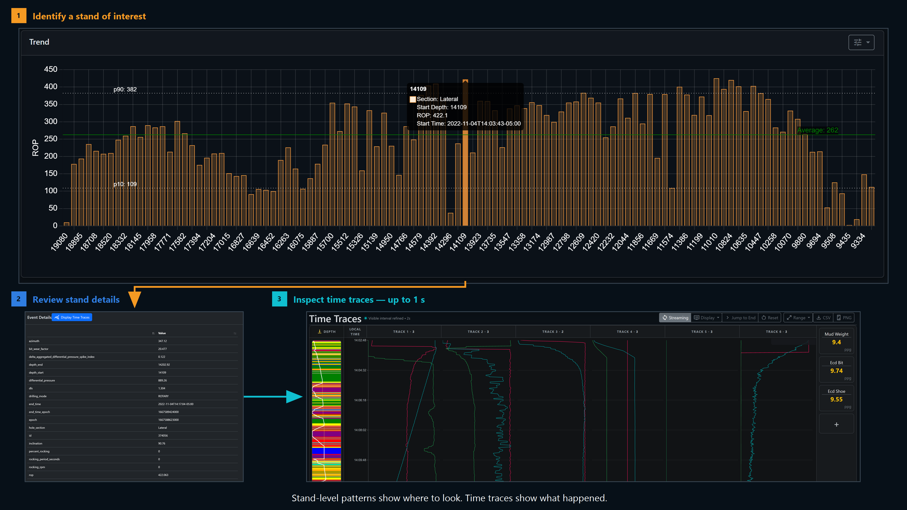
Stand-level KPIs show where to look; the linked time traces provide the detailed evidence.

The stand-level ROP chart makes broader patterns and stands of interest visible. Selecting a stand opens its interval details, including depth and operating context. From there, Display Time Traces opens the underlying interval at up to one-second frequency.

This preserves both analytical roles:

• aggregated stand KPIs for recognizing the broader pattern,
• time traces for investigating the evidence behind a selected stand.

Conclusion

Higher-frequency drilling data can reveal information that slower acquisition or aggressive averaging simply cannot preserve.

That makes it extremely valuable for the right applications.

But higher frequency also creates:

• more storage,
• more processing,
• more synchronization work,
• more noise,
• more opportunities to mistake raw variability for useful information.

The best drilling-data architecture therefore does not choose between:

high-frequency data

and:

aggregated data.

It preserves both roles.

Capture enough temporal detail to retain the important physical behavior.

Then transform that data deliberately according to the engineering question.

A two-second overpull may require second-level or faster evidence.

A fifty-hour bit-wear trend may be better represented by one robust statistic per stand.

A fleet comparison may need only formation-level distributions.

The correct question is not:

How fast can we sample the rig?

It is:

What is the fastest physical behavior this analysis needs to preserve, and what is the simplest data representation that still preserves it?

That is the difference between collecting more drilling data and extracting more engineering information from it.

---

References

1. Shahri, M., Wilson, T., Thetford, T., Nelson, B., Behounek, M., Ambrus, A., D'Angelo, J., and Ashok, P. Implementation of a Fully Automated Real-Time Torque and Drag Model for Improving Drilling Performance: Case Study. SPE-191426-MS, SPE Annual Technical Conference and Exhibition, Dallas, Texas, 2018.

2. Witt-Doerring, Y., Pastusek, P. P., Ashok, P., and van Oort, E. Quantifying PDC Bit Wear in Real-Time and Establishing an Effective Bit Pull Criterion Using Surface Sensors. SPE-205844-MS, SPE Annual Technical Conference and Exhibition, 2021.

3. Ashok, P., Ambrus, A., Ramos, D., Lutteringer, J., Behounek, M., Yang, Y. L., Thetford, T., and Weaver, T. A Step by Step Approach to Improving Data Quality in Drilling Operations: Field Trials in North America. SPE-181076-MS, SPE Intelligent Energy International Conference and Exhibition, Aberdeen, Scotland, 2016.

4. Shahri, M., Kutlu, B., Thetford, T., Nelson, B., Wilson, T., Behounek, M., Ambrus, A., and Ashok, P. Adopting Physical Models in Real-Time Drilling Application: Wellbore Hydraulics. SPE-191797-MS, SPE Liquids-Rich Basins Conference—North America, Midland, Texas, 2018.

5. Ambrus, A., Ashok, P., Thetford, T., Behounek, M., and others. Real-Time Detection of Drillstring Washouts and Mud-Pump Failures. IADC/SPE-189700-MS, 2018.