Separating Normal Drilling Variability from Meaningful Performance Changes

Real-time drilling signals are rarely stable. The analytical challenge is determining whether a change represents ordinary process variation, a new operating condition, or the beginning of a meaningful mechanical or operational event.

Torque increases by 8%.

Is something wrong?

ROP falls from 210 to 185 ft/hr.

Does that matter?

Standpipe pressure drops 70 psi.

Should anyone investigate?

There is no useful answer from the magnitude alone.

Drilling is inherently variable.

Measurements respond continuously to:

• formation,
• WOB,
• RPM,
• flow,
• bit condition,
• BHA behavior,
• trajectory,
• hole cleaning,
• rig activity,
• sensor behavior.

Even when the operation is completely healthy, the traces do not remain perfectly flat.

That creates one of the central problems in real-time drilling surveillance:

How do we distinguish ordinary variation from a meaningful change in the process?

An analytics system that reacts to every deviation becomes noisy.

An analytics system that smooths everything into a stable trend may become blind.

The useful region lies between those two extremes.

Published drilling research repeatedly encounters this problem.

SPE-166387 notes that drilling processes can vary significantly and unpredictably, which limits methods that assume the process itself is stable.[1]

SPE-186166 approaches the problem by evaluating both where a parameter currently lies and how it is moving over time.[2]

SPE-191426 provides a field example where averaging intended to make tripping data cleaner also reduced the magnitude of genuine overpull events.[3]

Together they illustrate an important principle:

Variability is not noise by definition.

Sometimes the variability is the engineering information.

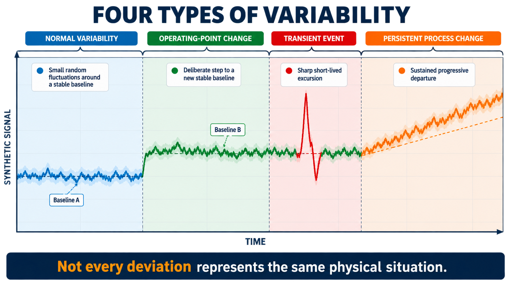
Real-time surveillance must distinguish ordinary variability, changes in operating context, short transients, and sustained changes in the drilling process.

A Fixed Value Is Rarely the Right Definition of Normal

Suppose normal surface torque is defined as:

$$T = 15,000 \pm 2,000\ ft\text{-}lb$$

That might work for one interval.

Then:

• inclination increases,
• lateral contact length increases,
• WOB changes,
• formation changes,
• hole cleaning deteriorates.

Healthy torque may now be:

$$19,000\ ft\text{-}lb$$

The sensor did not fail.

The process is not necessarily dysfunctional.

The baseline moved.

This is why drilling surveillance cannot usually define normality as one universal range.

A more useful concept is:

$$Normal = f( Operating\ State, Depth, Formation, Parameters, BHA, Well\ Condition )$$

Normal drilling is contextual.

Change from What?

Every change-detection problem implicitly requires a reference.

If current ROP is:

170 ft/hr

is that low?

Relative to what?

Possible references include:

• the previous minute,
• the previous stand,
• the previous 500 ft,
• other stands in the same formation,
• an offset-well distribution,
• a physics-based expectation.

These references answer different questions.

Previous few seconds

Useful for abrupt events.

Recent moving baseline

Useful for progressive deterioration.

Formation-specific history

Useful for performance benchmarking.

Physics-based model

Useful when the expected response can be calculated from current conditions.

Before classifying a change as abnormal, the reference itself should therefore be explicit.

Magnitude Alone Is Not Enough

Consider three hypothetical torque changes.

Case A

15,000 → 18,000 ft-lbf instantly.

Then returns to 15,000 ten seconds later.

Case B

15,000 → 18,000 ft-lbf after WOB was deliberately increased by 30%.

Case C

15,000 → 18,000 ft-lbf gradually over 20 minutes while all major surface set points remain stable.

The magnitude is identical:

$$\Delta T = 3,000\ ft\text{-}lb$$

But the engineering interpretation is very different.

Case A may be a transient.

Case B may be an expected response.

Case C may indicate a developing mechanical change worth investigating.

A meaningful detector therefore needs more than:

$$|x-x_{baseline}| > threshold$$

It needs context.

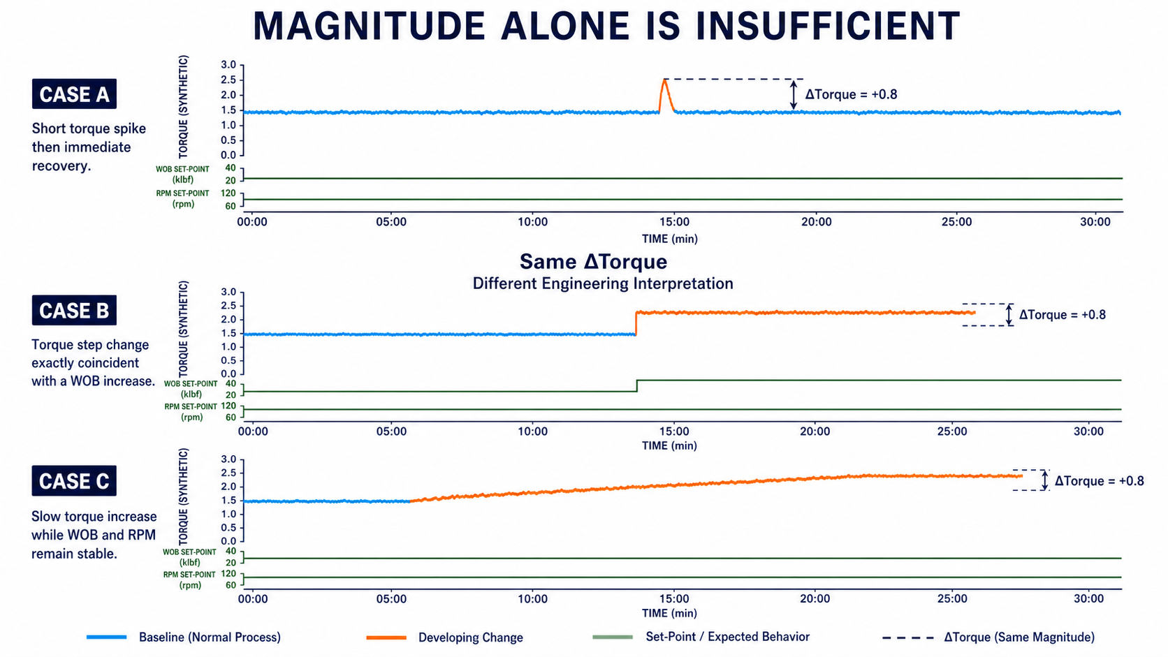
The same torque change can represent a short transient, an expected response to a WOB change, or a developing process change.

Location and Movement Describe Different Information

SPE-186166 provides a useful conceptual distinction.

The methodology represents drilling attributes using two broad types of features:

location

and

movement.

A location feature asks something like:

Is the current value low, normal, or high?

A movement feature asks:

Is the value increasing, decreasing, constant, or erratic?

Those are different pieces of evidence.

Suppose torque is high.

But it has been high and stable for the previous hour.

That is different from:

torque being normal and suddenly climbing.

Likewise, a moderate ROP may not be concerning if it is stable in the current formation.

A rapidly falling ROP may deserve more attention even before the absolute value becomes unusually low.

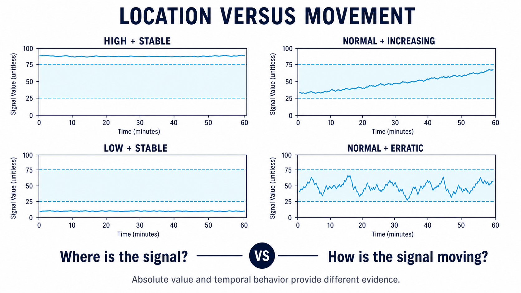
A signal's absolute level and its direction of movement provide different information about the drilling process.

The Baseline Should Move More Slowly Than the Event

Suppose we estimate normal ROP with a rolling average.

If the average adjusts too quickly, a real deterioration can become part of the new normal almost immediately.

The detector sees:

ROP decreases.

The baseline follows it downward.

The residual disappears.

No sustained anomaly remains.

Conversely, if the baseline changes too slowly, a legitimate formation transition can appear abnormal for hours.

There is therefore a basic design requirement:

The baseline must adapt slowly enough to preserve meaningful departures, but quickly enough to follow genuine changes in operating context.

There is no universal window that solves this.

The appropriate scale depends on the physics.

Window Length Defines What "Change" Means

Imagine calculating average torque using three possible windows.

5 seconds

Very responsive.

Also very noisy.

2 minutes

Less sensitive to individual spikes.

Useful for sustained short-term behavior.

30 minutes

Excellent for long trends.

Poor for rapidly developing events.

Each window produces a different interpretation of the same signal.

This is why window selection should begin with:

What physical event are we trying to detect?

not:

What smoothing setting makes the chart look nicest?

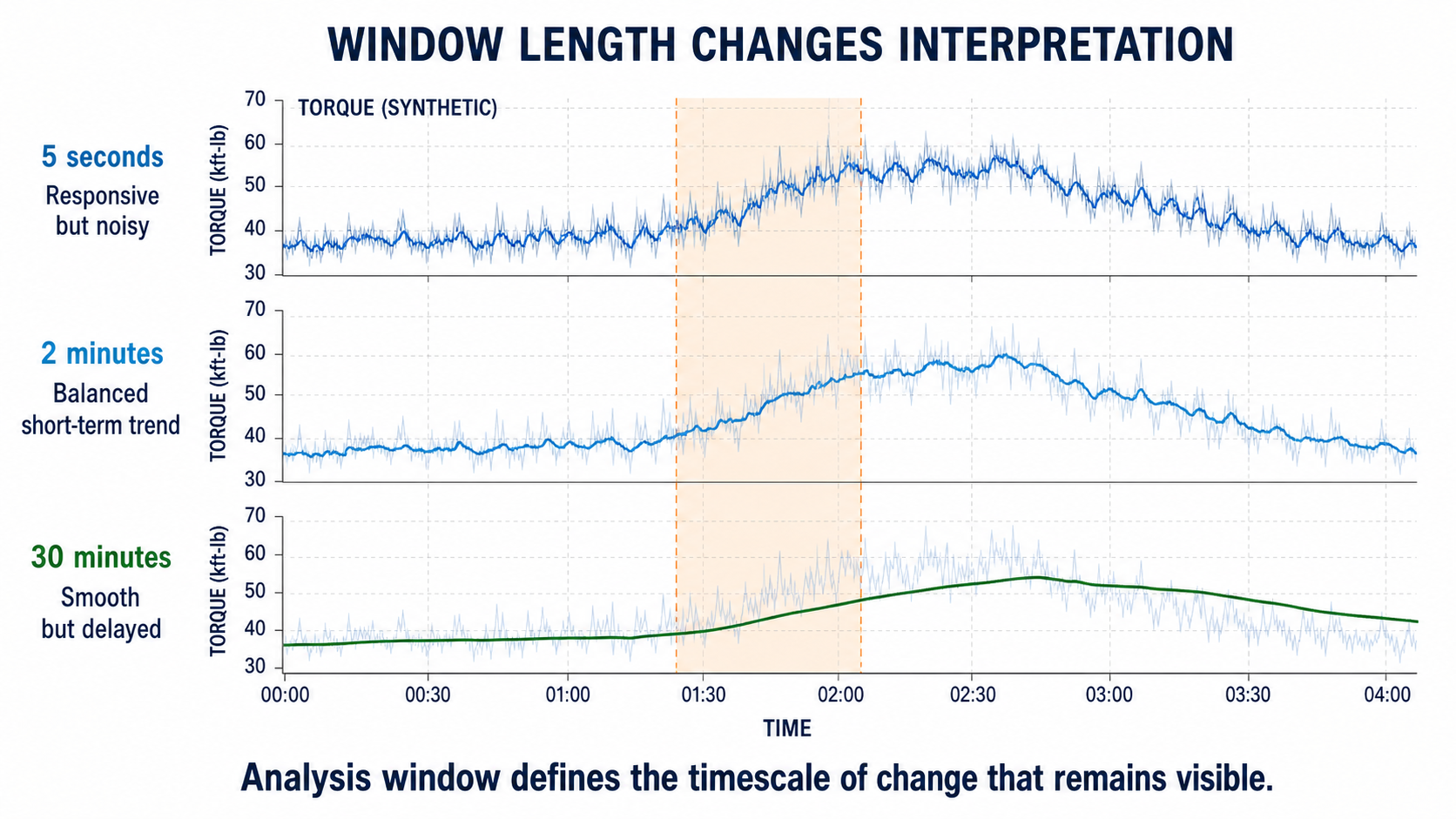
The analysis window determines which timescale of change remains visible.

Averages Can Hide Exactly What Matters

SPE-191426 provides a very practical field example.

During development of automated torque-and-drag surveillance, hook-load data was averaged by depth.

The averaging made the data cleaner.

But the full magnitude of overpull events was no longer visible.

The authors progressively reduced the averaging interval and ultimately removed the averaging for the relevant event-detection use case so that the full overpull could be retained.[3]

This is a broadly applicable lesson.

A filter that is excellent for estimating:

normal friction trend

may be poor for detecting:

short mechanical overpull.

Likewise:

a filter appropriate for long-term bit degradation may suppress:

a short torsional event.

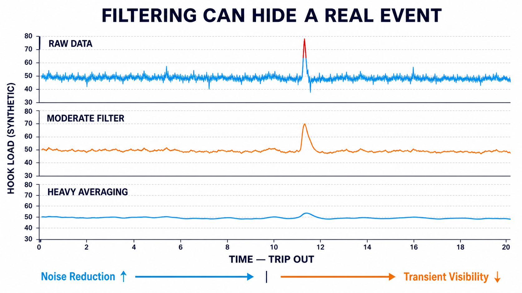
Smoothing reduces variance but can also reduce the apparent magnitude of genuine short-duration events.

Noise and Variability Are Not the Same Thing

These terms are often used interchangeably.

They should not be.

Measurement noise

variation caused by the sensing or acquisition process.

Process variability

real variation in the physical drilling system.

For example, small rapid torque fluctuations may reflect:

• sensor noise,
• actual torsional dynamics,
• or both.

Eliminating all variation can therefore remove legitimate physical behavior.

The goal of preprocessing is not:

make every signal smooth.

It is:

remove variation that is irrelevant to the engineering question while retaining variation that contains physical information.

Context Changes Should Reset the Comparison

Suppose ROP has been stable for an hour.

Then the driller changes:

• WOB from 28 to 38 klbf,
• RPM from 100 to 135.

ROP rises sharply.

A naive change detector flags:

ROP anomaly.

But the process was intentionally changed.

This suggests that certain contextual transitions should either:

• reset the baseline,
• create a new baseline population,
• or temporarily suspend the comparison.

Examples include:

• major parameter changes,
• formation transition,
• BHA change,
• rotary-to-slide transition,
• bit change,
• pump configuration change.

SPE-166387 gives a drilling-specific example of this general issue: changing mud-pump liners or pistons can alter the physical process while software may still be operating with stale assumptions, creating a discrepancy that could be mistaken for a sensor problem.[1]

The underlying principle is:

A process change should not automatically be treated as a process failure.

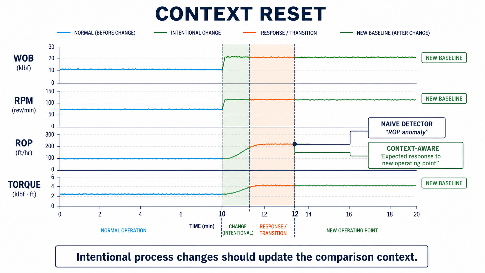
Intentional parameter changes should update the comparison context before the resulting drilling response is classified.

Rig State Is One of the Strongest Context Boundaries

Consider torque behavior during:

• drilling,
• reaming,
• rotating off bottom.

The normal range is different in each state.

Likewise, hook-load behavior during:

• pick-up,
• slack-off,
• static suspension

represents different mechanics.

SPE-166387 discusses how hook-load behavior during reaming can appear counterintuitive because of sheave friction and the influence of drillstring rotation.[1]

A generic threshold detector may interpret perfectly valid behavior as abnormal simply because the operating state changed.

This reinforces the architecture from the rig-state article:

$$Raw\ Data \rightarrow Rig\ State \rightarrow State\ Specific\ Baseline \rightarrow Change\ Detection$$

A New Formation Is Not an Anomaly

Suppose MSE increases abruptly at 12,700 ft.

At the same depth:

• ROP decreases,
• torque increases,
• gamma response changes.

One interpretation is:

drilling dysfunction.

Another is:

formation became harder.

SPE-186166 explicitly notes that formation changes, hole cleaning, hydraulics, and control-system behavior can all affect drilling-performance indicators.[2]

This is why drilling analytics benefits from combining:

behavioral change

with:

physical context.

Without context, every departure tends to look like a problem.

Persistence Adds Evidence

A ten-second change and a thirty-minute change should not normally carry equal weight.

Consider ROP.

A short dip may occur because of:

• a hard streak,
• toolface correction,
• temporary parameter transition.

A sustained reduction across multiple stands is a stronger signal that something material has changed.

A useful generic formulation is:

$$Meaningful\ Change = Magnitude + Duration + Context$$

Persistence does not prove causation.

It increases the evidence that the event is not simply a momentary fluctuation.

But Persistence Can Also Hide Sudden Events

This requires nuance.

Some events matter precisely because they are short.

Examples:

• severe overpull,
• motor stall,
• abrupt pressure loss,
• shock event.

Requiring a condition to persist for ten minutes would be inappropriate.

This means there are at least two broad surveillance classes.

Transient-event detection

Optimized to preserve short, high-magnitude behavior.

Process-change detection

Optimized to identify persistent departure from a baseline.

One algorithm should not necessarily be expected to do both.

Abrupt and Gradual Changes Are Different Problems

Consider bit performance.

A bit may:

Fail abruptly

ROP drops and never recovers.

Degrade gradually

ROP slowly declines over many stands.

SPE-205844 observed both longer-term baseline behavior and distinct departures associated with bit failure in its field dataset.[4]

The study used stand-level median values to reduce local noise, then examined how the wear indicator evolved against depth.

A sudden departure from the previous trend became more meaningful than the absolute value alone.

That concept generalizes nicely:

For progressive processes, departure from an established trajectory may be more useful than crossing one universal threshold.

Multiple Signals Can Increase Confidence

Suppose ROP drops 20%.

That may have many explanations.

Now suppose simultaneously:

• torque increases,
• MSE increases,
• differential pressure changes,
• parameter set points remain constant.

The evidence is stronger that the drilling process changed materially.

This does not automatically identify the cause.

It reduces the chance that one channel is reacting to ordinary local variation.

A useful principle is:

$$Confidence \uparrow \quad when\ independent\ evidence\ agrees$$

This is one reason probabilistic and relational drilling models can be useful.

They allow several pieces of imperfect evidence to contribute to one interpretation rather than requiring one sensor to tell the whole story.

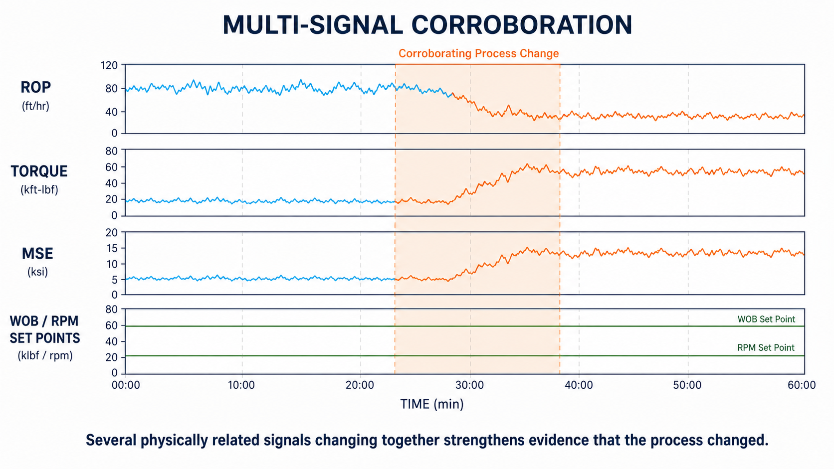
Several physically related signals changing together strengthen the evidence that the process changed without identifying the cause.

Correlated Signals Are Not Necessarily Independent Evidence

There is an important caution.

Suppose:

• ROP falls,
• MSE rises.

These may look like two separate pieces of evidence.

But ROP is already part of the MSE calculation.

The signals are mathematically related.

Counting them as fully independent observations can exaggerate confidence.

The same issue occurs when analytics combine multiple derived quantities built from the same source channels.

A mature surveillance system should understand:

• which signals are measured,
• which are derived,
• which share inputs.

Five indicators do not necessarily mean five independent observations.

Model Residuals Can Create a Better Baseline

Sometimes the expected value can be calculated.

For example:

$$Residual = Measurement - Model\ Prediction$$

Suppose SPP increases because pump rate increased.

Absolute pressure changed substantially.

But a hydraulic model also predicts a similar increase.

The residual may remain small.

No meaningful hydraulic anomaly exists.

Later:

pump rate is unchanged,

but measured SPP progressively falls below modeled pressure.

Now the residual grows.

That is more informative than pressure magnitude alone.

This turns change detection into:

Is the operation changing more than the physics predicts it should?

rather than:

Is this sensor moving?

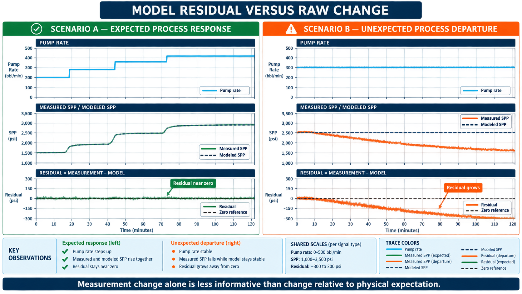
A model residual separates an expected pressure response from a departure that the current operating conditions do not explain.

Historical Distributions Can Define a Dynamic Envelope

The percentile article described historical P10–P90 ranges.

Those distributions can also support change detection.

Suppose comparable stands in this formation historically show:

Torque:

• P25 = 15.2 klbf-ft
• P50 = 16.0
• P75 = 16.8
• P90 = 17.6

The current well runs around:

16.2

for several stands.

Then:

17.3
17.8
18.2
18.7

The first high value may be ordinary variation.

Several consecutive stands moving above the historical envelope provide stronger evidence of a changing condition.

This combines:

distribution position

with:

movement

and:

persistence.

That is much more useful than any one of them alone.

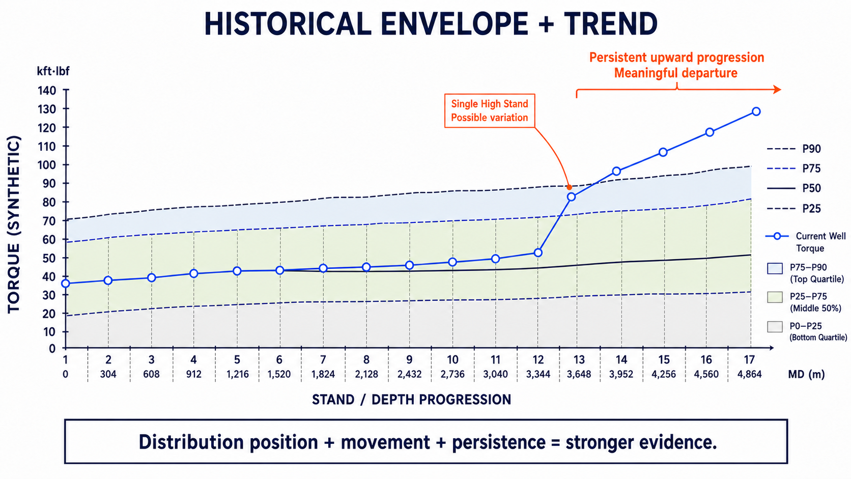
A sustained departure from an established trend can be more informative than a universal absolute threshold.

Beware of a Baseline Built from Mixed Conditions

A baseline is only as meaningful as the population behind it.

Suppose historical torque distributions combine:

• vertical,
• curve,
• lateral,
• rotary,
• reaming.

The resulting range may be extremely broad.

Almost nothing will ever look abnormal.

The opposite can happen if the baseline is too narrow.

A distribution built from one short interval may classify ordinary well-to-well variability as anomalous.

A good baseline therefore needs to be:

specific enough to be physically comparable

but:

broad enough to represent legitimate variation.

Baseline Quality Can Be Thought of as a Bias-Variance Problem

This provides a useful statistical analogy.

Very broad baseline

High variation.

Few false alarms.

May miss meaningful changes.

Very narrow baseline

Low variation.

Highly sensitive.

May flag every small difference.

The analyst is balancing:

sensitivity

against:

specificity to normal operation.

There is no universal answer because the cost of missing an event varies by application.

Do Not Train the Baseline on the Failure

Suppose a gradually deteriorating signal is continuously incorporated into a rolling historical window.

Eventually:

the abnormal behavior becomes the baseline.

This is sometimes called baseline contamination.

Operationally, it means the detector forgets that anything changed.

A surveillance system may therefore need rules governing when baseline learning is:

• active,
• frozen,
• reset.

For example:

once an event is suspected, the previous healthy baseline can be preserved for comparison until the condition resolves.

A Practical Example

Consider a hypothetical lateral.

For the previous 1,000 ft:

• WOB ≈ 34 klbf
• RPM ≈ 125
• torque median ≈ 16.0 klbf-ft
• rotary ROP ≈ 205 ft/hr.

Normal stand-to-stand variation is:

• torque: ±0.8 klbf-ft
• ROP: roughly ±20 ft/hr.

Stand 1

Torque:

16.7

ROP:

195

Nothing remarkable.

Stand 2

Torque:

17.1

ROP:

188

Still within plausible variation.

Stand 3

Torque:

17.8

ROP:

176

Now both signals are moving.

Stand 4

Torque:

18.4

ROP:

160

Stand 5

Torque:

19.0

ROP:

151

The key evidence is not simply:

Torque > 18

or:

ROP < 170.

It is:

• operating parameters are stable,
• torque is progressively rising,
• ROP is progressively falling,
• the pattern persists across multiple stands.

Now imagine gamma also changes at Stand 3.

The interpretation becomes less clear.

Perhaps formation changed.

That does not make the signal irrelevant.

It changes the question from:

Is drilling deteriorating?

to:

Is this deterioration expected from the formation change, or is there additional dysfunction?

That is what contextual surveillance should do.

What Makes a Change Operationally Meaningful?

A practical change assessment might consider six dimensions.

Magnitude

How far did the signal move?

Rate

How quickly did it move?

Persistence

How long has the change remained?

Context

Did parameters, formation, or rig state change?

Corroboration

Do other physically relevant signals support the same interpretation?

Consequence

Would this change alter an engineering decision?

The final item matters.

A statistically significant change can still be operationally irrelevant.

Statistical Significance Is Not Engineering Significance

With enough 1-Hz drilling data, very small differences can become statistically detectable.

Suppose median torque changes from:

15.00

to:

15.15 klbf-ft.

With tens of thousands of samples, a statistical test may confidently conclude that the distributions differ.

Does the drilling engineer care?

Maybe not.

The physical magnitude may be negligible.

This is why real-time analytics should ask:

$$Is\ the\ change\ statistically\ credible?$$

and:

$$Is\ the\ change\ physically\ meaningful?$$

and:

$$Is\ the\ change\ operationally\ actionable?$$

Those are three different questions.

A Useful Change-Detection Workflow

A practical workflow might be:

1. Identify the operating state

Do not compare incompatible operations.

2. Establish the relevant baseline

Possible basis:

• recent healthy operation,
• comparable historical interval,
• physics model,
• offset distribution.

3. Measure current position

Where is the current value relative to normal?

4. Measure movement

Is it:

• increasing,
• decreasing,
• stable,
• erratic?

5. Check persistence

One sample?

One stand?

Several stands?

6. Check context changes

Did any of these change?

• WOB
• RPM
• flow
• formation
• BHA
• rig state

7. Seek corroboration

Which other channels should change if this interpretation is correct?

8. Preserve the raw data

Do not let smoothing remove the physical event.

9. Assign uncertainty

If multiple explanations remain plausible, say so.

10. Escalate only when the change matters

An interesting data change does not automatically require an operational alert.

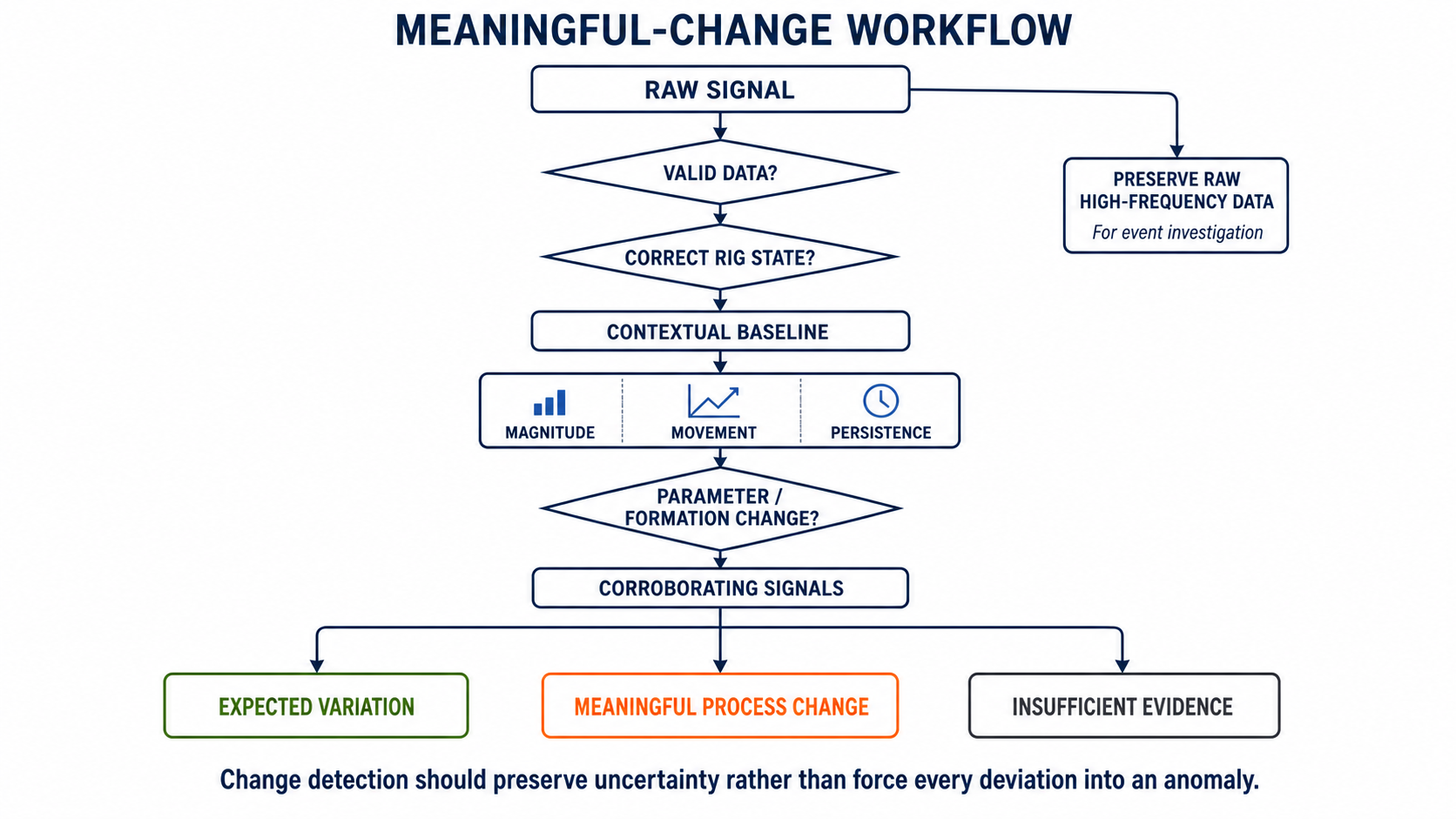
Meaningful change detection combines magnitude, movement, persistence, operating context, and corroborating evidence while preserving uncertainty.

A Good Output Is Not Just "Anomaly"

An anomaly score alone leaves the engineer with another interpretation problem.

A more useful output might say:

Performance Change Detected

Observed

• rotary ROP has declined across four consecutive stands,
• torque has increased across the same interval,
• WOB/RPM/flow have remained approximately stable.

Context

• no rig-state transition detected,
• no known parameter change,
• formation marker nearby.

Interpretation

• evidence supports a meaningful change in drilling response,
• formation transition and mechanical dysfunction remain competing explanations.

This is much more useful than:

Anomaly Score = 0.83

The goal is to preserve engineering meaning.

DrillingMetrics Example: Progressive ROP Departure

The synchronized depth view below shows current-well ROP progressively separating from both the offset response and its earlier baseline. RPM remains fixed at approximately 70 rpm, while WOB remains within a broadly comparable operating range.

Near 9,150 ft, the discontinuity and BHA marker correspond to the bit trip performed to pull and replace the bit. The preceding ROP decline is evidence of a meaningful performance change, but the traces alone do not establish its cause.

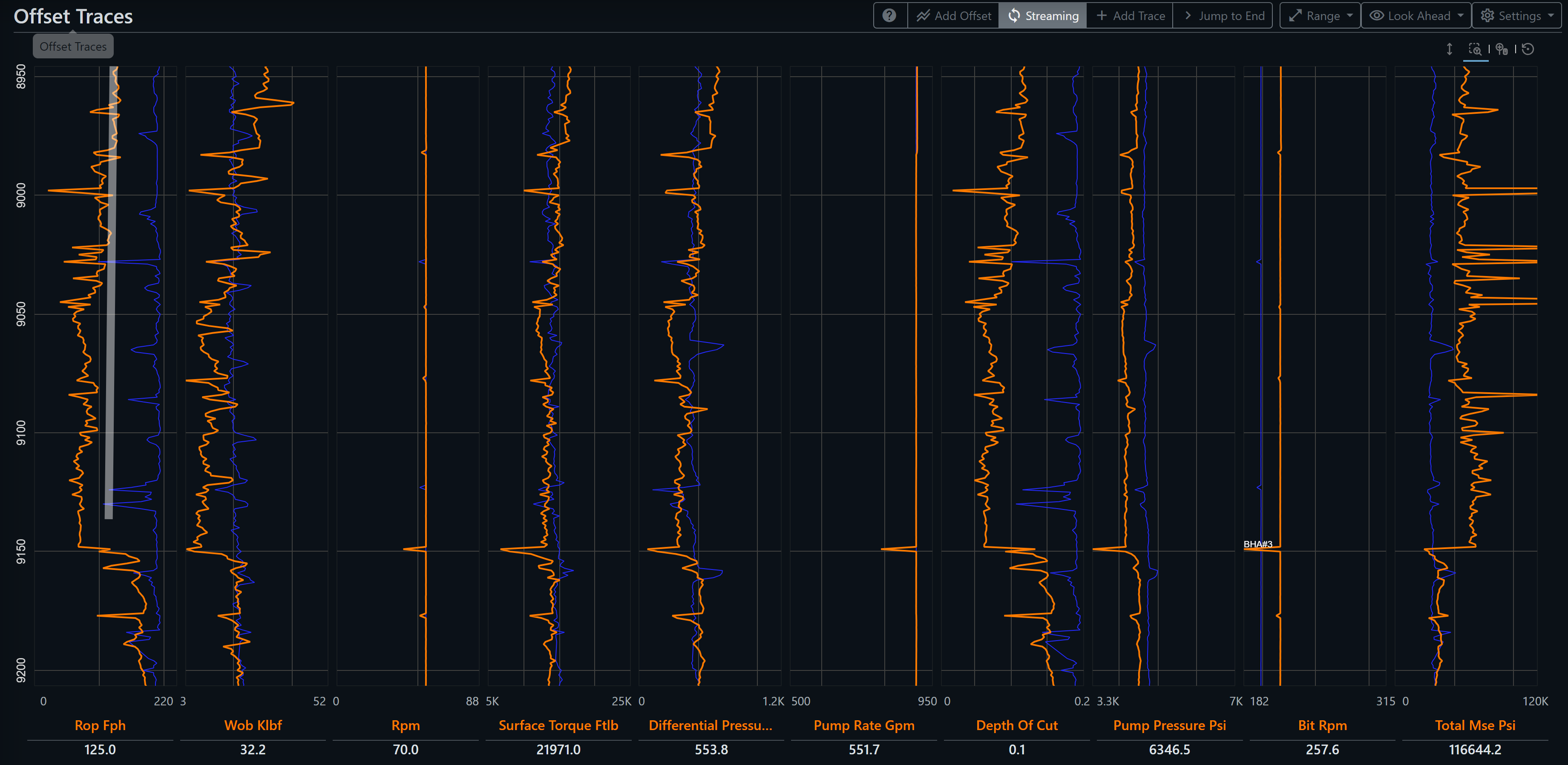
Current-well ROP progressively separates from the offset response and its earlier baseline before the bit trip near 9,150 ft. The synchronized tracks provide evidence of a meaningful performance change without establishing its cause from ROP alone.

The Baseline Is an Engineering Assumption

This may be the most important lesson.

Every statement that says:

this is abnormal

implicitly says:

this is what we believed normal should have been.

That normal reference might come from:

• recent history,
• offsets,
• a model,
• a distribution,
• an engineering threshold.

Each contains assumptions.

Therefore the baseline itself deserves scrutiny.

If the baseline is wrong, the anomaly is wrong.

Real-Time Surveillance Is Mostly About Comparing Expectations with Reality

Many drilling analytics can ultimately be expressed as:

$$Observed - Expected$$

Sensor validation:

Is the measurement consistent with what related sensors and physics suggest?

Torque and drag:

Is hook load consistent with the calibrated mechanical model?

Offset benchmarking:

Is current performance consistent with comparable historical wells?

Bit surveillance:

Is the current trend departing from the expected wear progression?

Hole cleaning:

Is the recent operational history consistent with favorable hole condition?

The sophistication lies largely in defining:

expected.

Conclusion

Real drilling data is not supposed to be perfectly stable.

Healthy drilling contains variation.

The challenge is deciding when that variation becomes evidence that the system itself has changed.

The strongest answer rarely comes from one threshold.

It comes from combining:

• a physically meaningful baseline,
• signal magnitude,
• movement,
• persistence,
• operating context,
• corroborating evidence.

Equally important, the method should preserve the timescale of the event.

Smoothing that is ideal for long-term trend analysis may erase short mechanical events.

A detector optimized for spikes may overreact to routine variation.

There is therefore no universal definition of a meaningful drilling change.

The engineering question determines:

• the baseline,
• the window,
• the population,
• the evidence required.

The objective of real-time surveillance is not to eliminate variability from the data.

It is to determine which variability is simply part of drilling—and which variability is telling us that something important has changed.

---

References

1. Ambrus, A., Ashok, P., and van Oort, E. Drilling Rig Sensor Data Validation in the Presence of Real-Time Process Variations. SPE-166387-MS, SPE Annual Technical Conference and Exhibition, New Orleans, Louisiana, 2013.

2. Ambrus, A., Ashok, P., Chintapalli, A., Ramos, D., Behounek, M., Thetford, T. S., and Nelson, B. A Novel Probabilistic Rig Based Drilling Optimization Index to Improve Drilling Performance. SPE-186166-MS, SPE Offshore Europe Conference & Exhibition, Aberdeen, United Kingdom, 2017.

3. Shahri, M., Wilson, T., Thetford, T., Nelson, B., Behounek, M., Ambrus, A., D'Angelo, J., and Ashok, P. Implementation of a Fully Automated Real-Time Torque and Drag Model for Improving Drilling Performance: Case Study. SPE-191426-MS, SPE Annual Technical Conference and Exhibition, Dallas, Texas, 2018.

4. Witt-Doerring, Y., Pastusek, P. P., Ashok, P., and van Oort, E. Quantifying PDC Bit Wear in Real-Time and Establishing an Effective Bit Pull Criterion Using Surface Sensors. SPE-205844-MS, SPE Annual Technical Conference and Exhibition, 2021.