When “Unable to Determine” Is the Correct Output in Drilling Analytics

An analytical system that always returns a diagnosis may appear decisive, but it can be less reliable than one that recognizes when the available measurements, context, or model evidence are insufficient.

Imagine a drilling surveillance system evaluating a pressure anomaly.

It sees:

• standpipe pressure decreasing,
• pump rate approximately constant,
• modeled pressure higher than measured pressure.

Those observations are consistent with a problem somewhere in the circulating system.

The software now has to choose between:

Drillstring washout

and:

Mud-pump failure

But the flow-out sensor is unavailable.

Should the system choose the more probable explanation?

Should it report whichever condition occurred more frequently in the historical dataset?

Should it return:

Washout — 54%

and:

Pump Failure — 46%

and let the user assume that washout is the diagnosis?

There is another possibility:

The available evidence is sufficient to identify a hydraulic abnormality, but insufficient to determine which failure mode is responsible.

That answer may be less satisfying.

It is also more technically defensible.

This problem appears throughout drilling analytics.

Sensors fail.

Context is missing.

Models contain uncertainty.

Several drilling conditions produce overlapping signatures.

Operating state changes the meaning of measurements.

And some events simply cannot be uniquely diagnosed from the available surface data.

A mature analytical system therefore needs more than two outputs:

$$\text{Yes}$$

and:

$$\text{No}$$

It also needs:

$$\text{Unable to Determine}$$

That third state is not evidence that the analytics failed.

Sometimes it is evidence that the analytics correctly understands the limits of the information available to it.

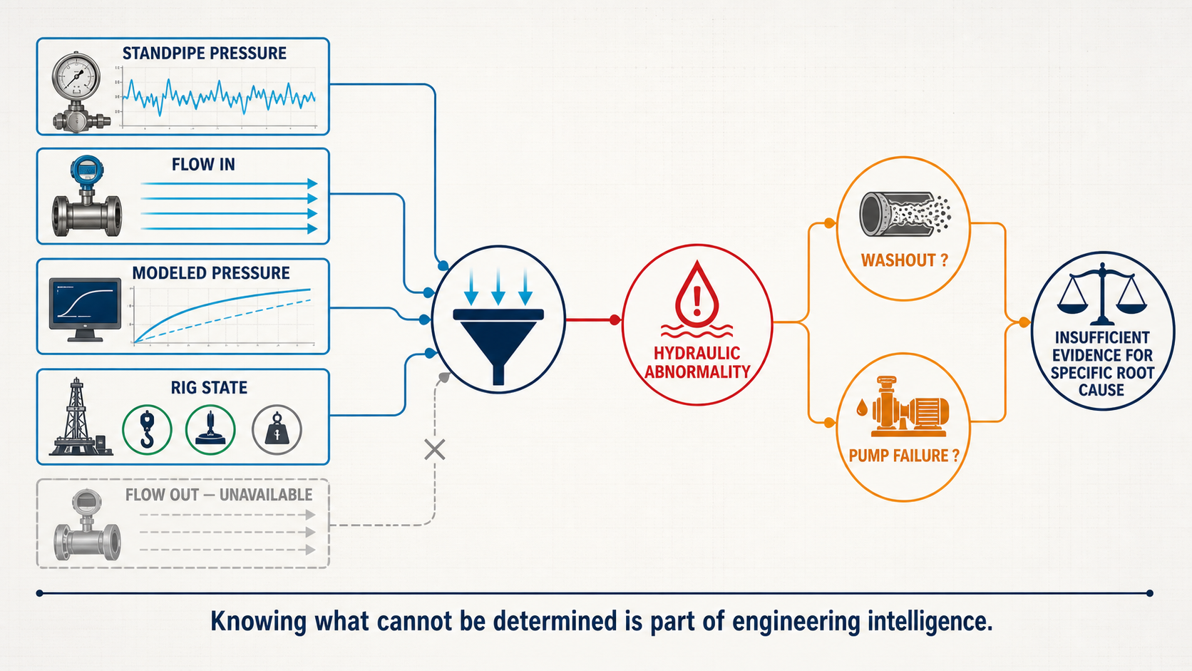
A reliable analytical system should match the specificity of its conclusion to the strength of the available evidence.

Binary Classification Is Attractive

Many analytical problems are naturally framed as binary questions.

Is the sensor healthy?

Yes / No.

Is there a washout?

Yes / No.

Is the rig drilling?

Yes / No.

Is hole cleaning adequate?

Yes / No.

Binary outputs are easy to:

• display,
• alert on,
• automate,
• summarize.

They are also easy to misunderstand.

The underlying evidence rarely exists in perfectly binary form.

Suppose a pressure sensor differs from a physics-based estimate.

That discrepancy could mean:

• the sensor is biased,
• the process changed,
• the model is wrong,
• the contextual inputs are wrong,
• several of these occurred simultaneously.

A forced binary classifier may still produce:

Sensor Fault

or:

Sensor Healthy.

But the information may not justify either conclusion confidently.

A Third State Changes the Logic

Instead of:

$$Output \in { Normal,\ Fault }$$

consider:

$$Output \in { Normal,\ Fault,\ Unable\ to\ Determine }$$

Now the model can distinguish:

Evidence supports normal

The available observations are sufficiently consistent with expected behavior.

Evidence supports fault

The observations provide adequate evidence for the fault interpretation.

Unable to determine

The system does not have enough reliable information to distinguish competing explanations.

This is a much more useful representation of engineering reality.

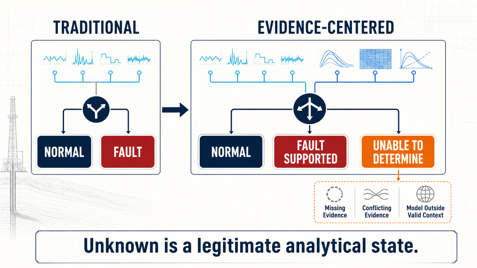
A three-state classifier preserves unable-to-determine as a legitimate output when evidence is missing, conflicting, or outside the model's valid context.

“Unknown” Is Not the Same as “Normal”

This distinction is critical.

Suppose the hook-load sensor stops transmitting.

The system can no longer calculate:

• hook-load trend,
• hook-load deviation,
• several derived mechanical indicators.

One possible implementation is to assign those missing features their default healthy state.

That would make the downstream model appear more confident that everything is normal.

But nothing became more normal.

The system simply lost information.

SPE-191426 describes a better approach in a real-time tripping-dysfunction model.

When hook-load data is unavailable, the hook-load trend feature cannot be calculated.

Rather than treating the missing feature as either:

constant

or:

erratic,

the feature is assigned an unknown state.

That prevents the network from placing excessive weight on evidence that does not exist.

This is a fundamental analytical principle:

Absence of evidence is not evidence of normal operation.

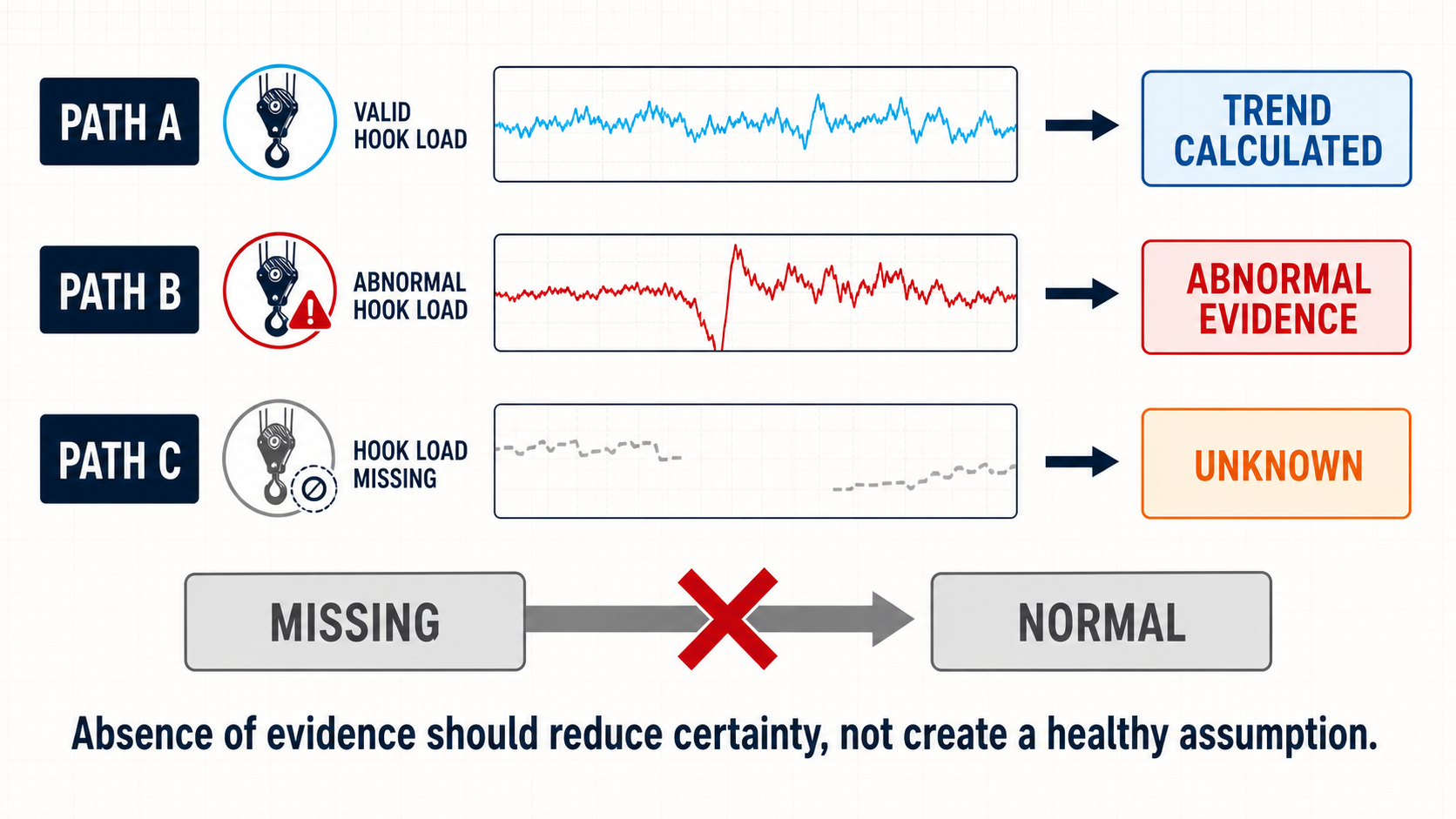
Missing hook-load data removes information; it does not support a normal-operation conclusion.

Unknown Is Also Not the Same as Fault

The reverse mistake is equally dangerous.

A missing sensor does not prove that the process itself is abnormal.

Suppose:

Flow Out = unavailable

during otherwise stable drilling.

The correct conclusion is not:

Flow anomaly detected.

The correct conclusion is:

Flow-out evidence is unavailable.

The process may still be operating normally.

The distinction between:

• missing measurement,
• faulty measurement,
• abnormal process

must remain explicit.

Public Drilling Research Already Uses This Principle

SPE-181076 describes a field-deployed sensor-validation system with several distinct output categories, including:

• OK,
• Missing,
• Outlier,
• Monitoring Possible Sensor Bias Fault,
• Unable to Determine Sensor Health,
• Bias Fault Detected.

The presence of the Unable to Determine category is important.

The paper explains that during some conditions and rig states, the Bayesian model simply does not contain sufficient information to reliably identify a sensor bias.

The model does not force an answer.

That is precisely what a trustworthy engineering system should do.

Rig State Can Determine Whether a Question Is Even Answerable

Consider torque.

During rotary drilling, torque contains information about the rotating drillstring and bit interaction.

During a connection:

surface RPM may be zero.

During a trip:

the mechanical interpretation changes again.

A sensor-validation or dysfunction model may therefore have strong evidence during one rig state and weak evidence during another.

This means:

$$Evidence\ Quality = f(Rig\ State)$$

The same measurement channel can be:

highly informative

in one operating state,

and:

nearly useless

for a particular diagnosis in another.

A reliable system should therefore be allowed to say:

This condition cannot currently be determined in this operating state.

That is better than producing a classification from an inappropriate population.

Diagnostic Specificity Should Follow Evidence

The hydraulic example makes this especially clear.

Suppose:

• measured pressure is below model,
• flow in is stable,
• pressure trend is persistently decreasing.

That may strongly support:

Circulating-System Abnormality

But washout and pump failure can share many of the same signatures.

Now add flow-out behavior.

Perhaps the two failure modes become easier to separate.

So we can think of diagnostic specificity as a hierarchy.

Level 1

Something unusual is happening.

Level 2

The abnormality appears hydraulic.

Level 3

The evidence supports a washout-or-pump-failure family.

Level 4

The evidence distinguishes one specific failure mode.

Each step requires more evidence.

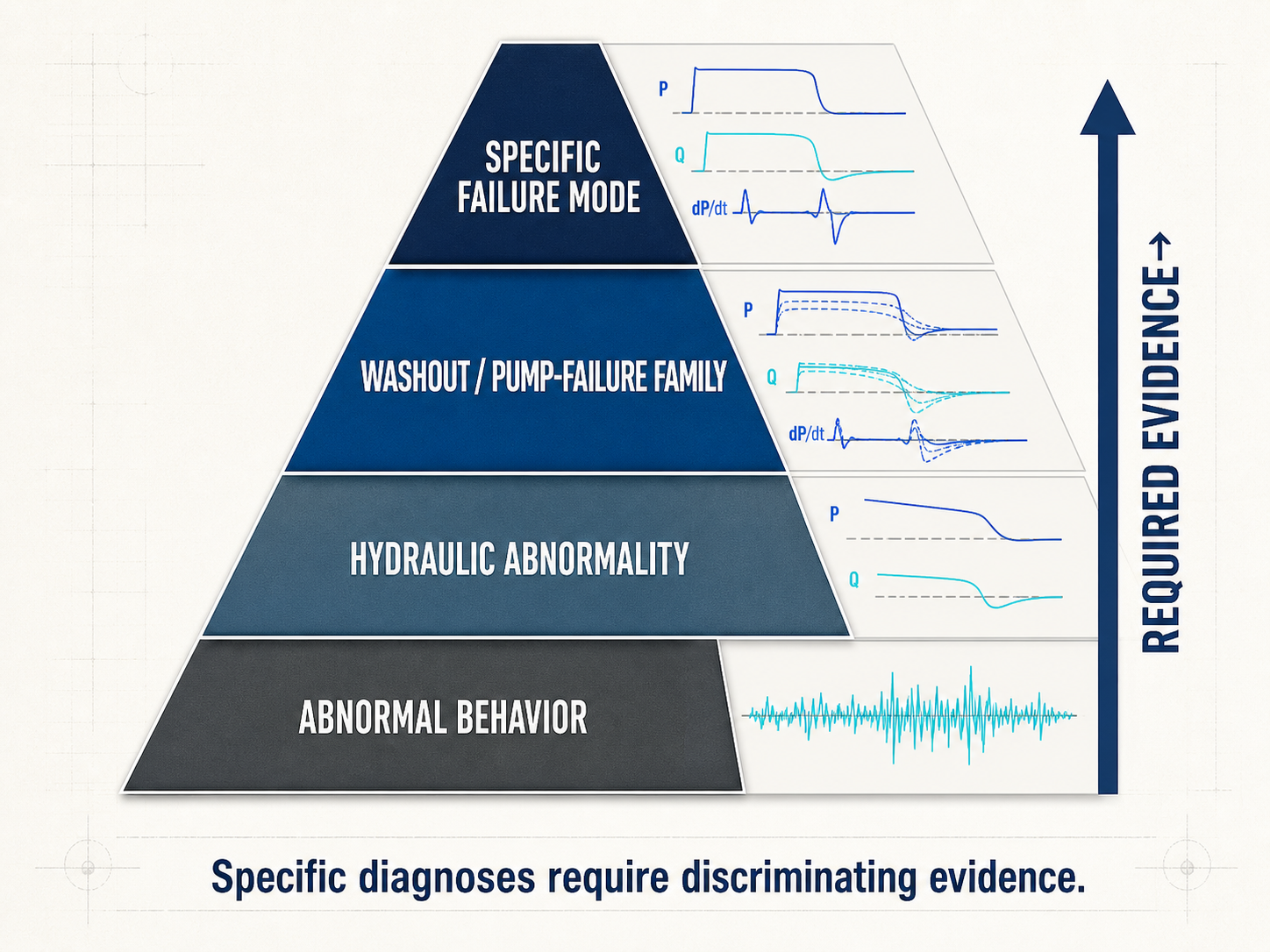
Each higher level of diagnostic specificity requires more discriminating evidence.

Broad-but-Correct Can Be Better Than Specific-but-Wrong

Suppose the available evidence indicates:

washout OR pump failure

with strong confidence.

A system that reports:

Hydraulic system abnormality—washout or pump failure should be investigated.

has provided useful information.

Another system reports:

Drillstring washout detected.

That is more specific.

It is also potentially wrong.

Specificity is valuable only when the evidence supports it.

This principle applies beyond hydraulics.

Torque and drag

The evidence may support:

abnormal drag

without proving:

cuttings bed at 14,200 ft.

Bit performance

The evidence may support:

bit effectiveness deteriorating

without proving:

shoulder-cutter thermal damage.

Hole cleaning

The evidence may support:

poor hole condition likely

without proving the exact cuttings-bed geometry.

Engineering analytics should therefore preserve the distinction between:

what was observed

and:

what is inferred.

Confidence Does Not Solve an Underdetermined Problem

A probability can make uncertainty look precise.

Suppose a system reports:

Washout 52%

Pump Failure 48%

Should the engineer treat washout as the diagnosis?

Probably not.

The difference may simply indicate that the evidence does not meaningfully distinguish the two.

A useful system might instead recognize:

$$|P_1-P_2| \approx 0$$

and communicate:

Specific root cause unresolved.

Probability does not eliminate ambiguity.

Sometimes probability is how ambiguity becomes visible.

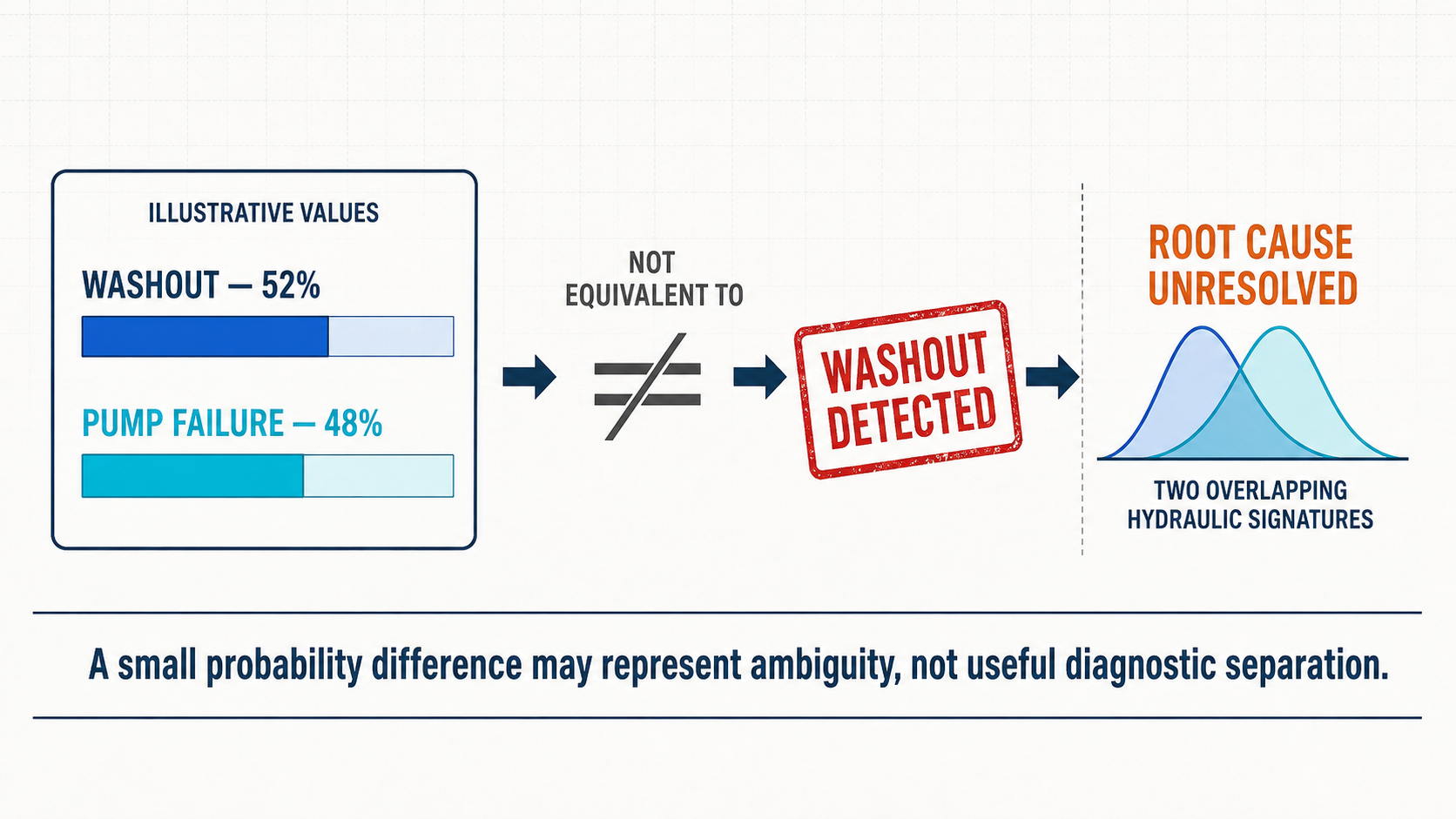
Illustrative 52% and 48% results represent unresolved root cause, not a supported washout diagnosis.

Missing Evidence Should Widen the Conclusion

Consider the same hydraulic case.

With flow-out measurement

The system has:

• pressure,
• flow in,
• flow out,
• model prediction,
• rig state.

A specific diagnosis may become possible.

Without flow-out measurement

The system still has evidence of abnormal hydraulic behavior.

But the missing discriminator should make the conclusion broader.

This is an important design principle:

When discriminating evidence disappears, diagnostic specificity should decrease.

It should not stay artificially constant.

Good Models Lose Confidence Gracefully

This is sometimes called graceful degradation.

Suppose an analytical system normally uses five evidence streams.

One becomes unavailable.

A brittle system may:

• stop entirely,
• silently substitute a default,
• continue producing the same confidence.

A better system changes its behavior proportionally.

Perhaps it moves from:

Specific fault likely

to:

Fault family likely

or:

Unable to distinguish cause.

If additional evidence disappears, it may eventually reach:

Unable to determine whether an abnormal event is present.

That progression mirrors the actual reduction in information.

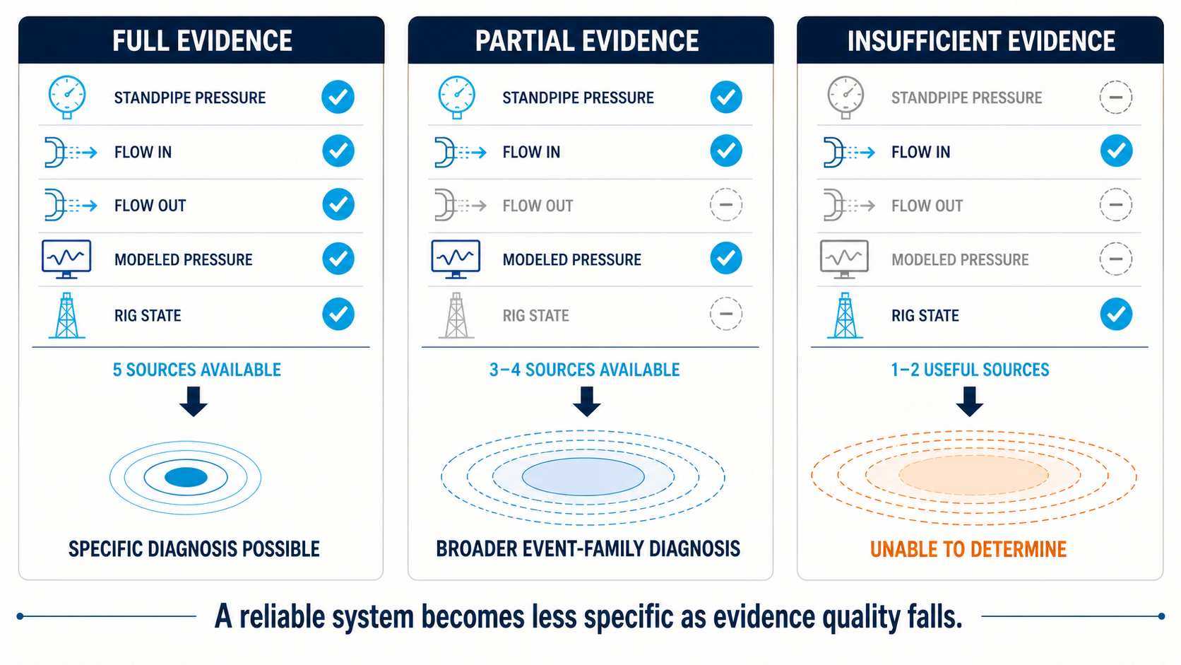
As useful evidence streams disappear, a reliable output should broaden from a specific diagnosis to an event family and eventually to unable to determine.

Model Uncertainty Matters Even When All Sensors Work

Missing data is not the only reason a system should abstain.

Suppose every sensor is functioning.

But the physical model itself has large uncertainty under the current conditions.

Examples might include:

• uncertain mud rheology,
• uncertain hole geometry,
• unknown washout,
• poor friction-factor calibration,
• uncertain bit condition.

Now the measurements may be precise while the expected model response is uncertain.

A disagreement between measurement and model is less meaningful when the model uncertainty band is broad.

SPE-181076 explicitly discusses uncertainty in both the sensor reading and the model prediction.

That is important because:

$$Measurement - Model$$

is only useful if we also understand uncertainty in both terms.

An Analytical Residual Is Not a Verdict

Suppose:

$$Residual = Measured - Expected$$

is large.

That tells us:

measurement and expectation disagree.

Possible explanations include:

• sensor fault,
• process fault,
• model error,
• contextual-data error.

The residual is evidence.

It is not automatically a diagnosis.

The same logic applies throughout the drilling analytics stack.

Conflicting Evidence Should Reduce Certainty

Consider a hypothetical stuck-pipe surveillance problem.

Evidence A:

Torque increasing

supports worsening hole condition.

Evidence B:

Hook-load behavior normal

does not.

Evidence C:

Hole-cleaning activity extensive

argues against severe accumulation.

Evidence D:

Flow below historical norm

may support concern.

What should the system do?

A poor implementation may choose whichever signal has the largest numerical score.

A stronger implementation represents the conflict.

Possible output:

Evidence is mixed. Current data does not support a confident hole-condition diagnosis.

This is not indecision.

It is an accurate representation of the state of knowledge.

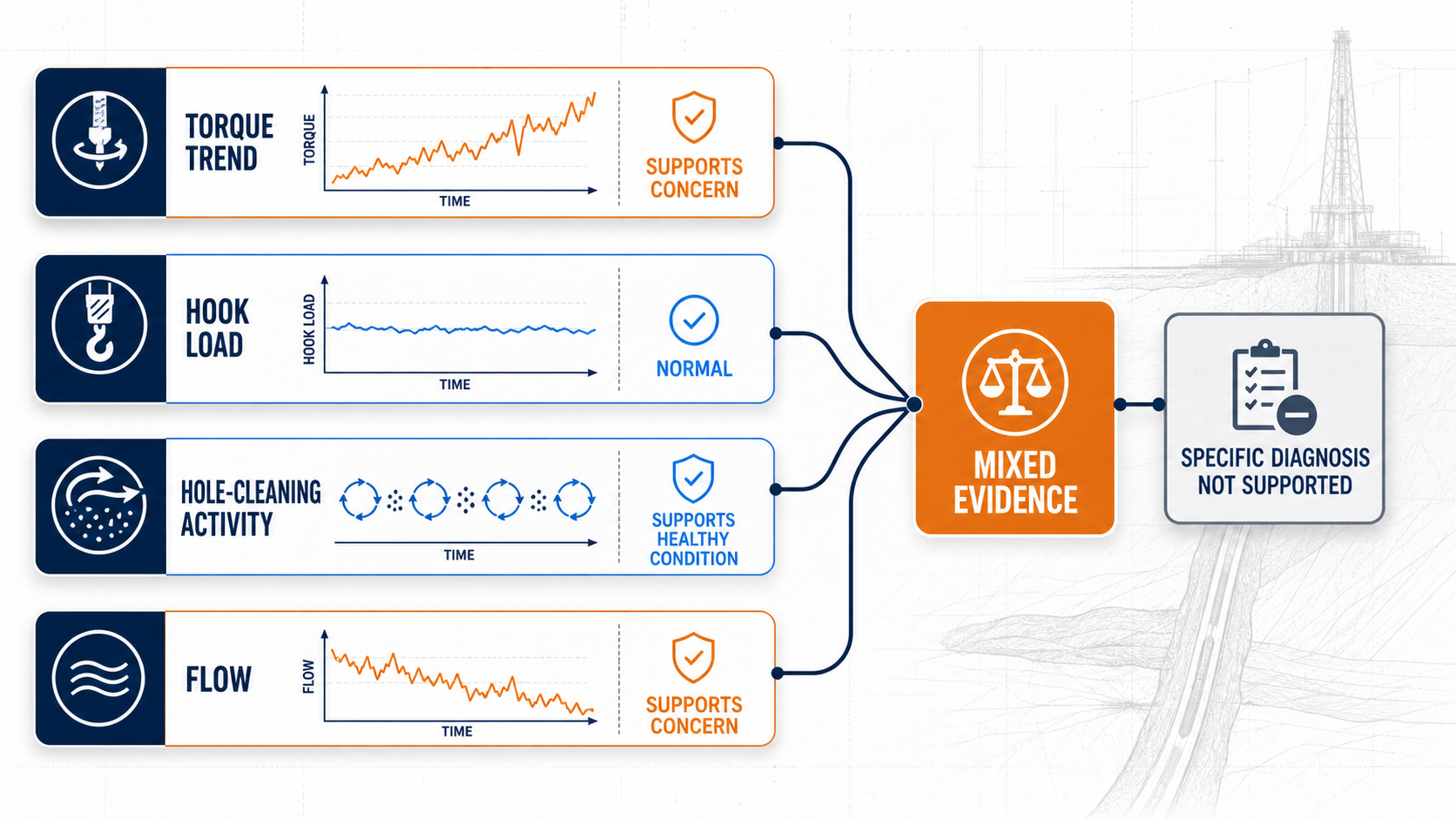
Conflicting evidence should remain visibly mixed when the available signals do not support a specific hole-condition diagnosis.

Several Weak Signals Do Not Necessarily Create One Strong Conclusion

There is also a dependency problem.

Suppose five analytical features are all derived partly from ROP.

ROP falls.

All five features deteriorate.

The system may appear to have five independent pieces of evidence.

It really has one important underlying change propagated through several calculations.

Therefore evidence strength should consider:

• provenance,
• shared inputs,
• dependency.

Five correlated indicators are not equivalent to five independent observations.

This becomes especially important in AI systems that summarize many derived KPIs.

“Unable to Determine” Should Explain Why

A bare message:

Unable to determine.

is not very useful.

A better result explains the limitation.

For example:

Unable to distinguish washout from pump failure because flow-out data is unavailable.

or:

Unable to assess hook-load trend because the hook-load channel has not updated for 45 seconds.

or:

Unable to compare current MSE with the historical baseline because the current formation has not been resolved.

The explanation converts uncertainty into an actionable next step.

The user now knows:

what information is missing.

Uncertainty Should Be Inspectable

A useful output could contain:

What is known

• pressure decreased,
• pump rate remained stable,
• model expected higher pressure.

What is missing

• flow-out measurement.

What can be concluded

• hydraulic abnormality is plausible.

What cannot be concluded

• washout versus pump failure cannot currently be distinguished.

What would reduce uncertainty

• restore flow-out measurement,
• inspect pump behavior,
• compare additional hydraulic evidence.

That is a much stronger decision-support output than simply:

Unknown.

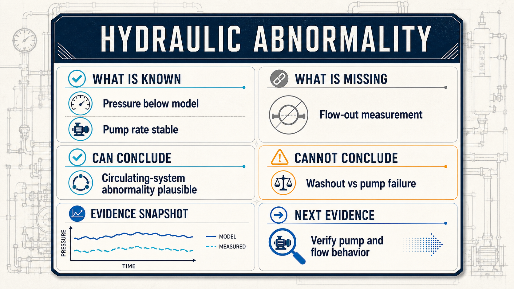
An evidence-centered output separates what is known, what is missing, what can be supported, and what remains unresolved.

The Best Analytics Can Separate Three Questions

Many systems combine these into one.

They should be separated.

Question 1 — Did something change?

This is change detection.

Question 2 — What class of problem does the evidence support?

This is classification.

Question 3 — What exact root cause occurred?

This is diagnosis.

The available evidence may support Question 1 strongly while supporting Question 3 poorly.

That is perfectly acceptable.

For example:

Yes, the hydraulic process changed.

Likely circulating-system fault.

Exact root cause unable to determine.

Each statement has a different level of certainty.

Decision Support Does Not Always Require Full Diagnosis

This is operationally important.

Suppose the system cannot distinguish:

• washout,
• pump degradation.

Can it still be useful?

Yes.

The appropriate immediate action may be:

investigate the circulating system.

A perfect root-cause diagnosis may not be necessary before the engineer begins checking:

• pump response,
• pressure behavior,
• flow measurements.

The best analytics therefore aims for:

the most specific conclusion required to support the next decision

rather than:

the most specific conclusion imaginable.

False Certainty Can Be More Expensive Than Explicit Uncertainty

Consider two systems.

System A

Produces a diagnosis on every event.

Operators frequently discover that the root cause was wrong.

System B

Sometimes reports:

Unable to distinguish

but when it gives a specific diagnosis, the evidence is stronger.

Which system will engineers trust longer?

Usually the second.

False precision has a cumulative credibility cost.

Once operators learn that:

specific does not mean reliable,

they begin ignoring the system.

This connects directly to alarm fatigue.

The problem is not only too many alerts.

It is too many alerts that claim more than the evidence supports.

The Same Principle Applies to Engineering AI

This becomes even more important with language models.

A language model is naturally optimized to produce an answer.

But an engineering assistant should not equate:

answer generation

with:

problem resolution.

Suppose an engineer asks:

Why is torque increasing?

Available data shows:

• torque rising,
• ROP falling,
• WOB stable.

But:

• formation data is unavailable,
• BHA context is incomplete,
• hole-cleaning history cannot be retrieved.

A conversational system can easily produce a plausible explanation:

The increase is likely caused by poor hole cleaning.

That may sound technically reasonable.

The evidence does not justify it.

A stronger answer is:

Torque is rising while WOB remains stable and ROP is declining, which confirms a change in drilling response. Current evidence is insufficient to distinguish formation change, hole condition, or mechanical dysfunction.

That answer is less dramatic.

It is much more useful.

LLM Abstention Should Be Evidence-Based

A reliable engineering assistant can implement the same three-state philosophy.

Answer supported

Evidence is sufficient.

Qualified answer

A conclusion is possible but assumptions or uncertainty must be stated.

Unable to determine

The available data cannot support the requested conclusion.

This does not mean an LLM should refuse frequently.

It means the threshold for specificity should depend on evidence quality.

Source Provenance Helps Determine Whether a Question Is Answerable

Suppose an AI system retrieves two conflicting mud weights.

DDR

12.0 ppg.

Real-time mud database

11.6 ppg.

Which is correct now?

Before calculating ECD, the system should resolve:

• timestamps,
• source freshness,
• well/wellbore,
• whether one value is planned versus actual.

If it cannot resolve the conflict, the correct output may be:

Current mud weight cannot be determined reliably from the available sources.

Running a precise hydraulic calculation with an arbitrary choice would produce false precision.

A Number of Decimal Places Does Not Represent Certainty

Consider:

ECD = 12.438 ppg

The display appears precise.

But perhaps:

• rheology is six hours old,
• hole size is uncertain,
• flow is measured accurately,
• model error is ±0.3 ppg.

The meaningful engineering statement may actually be closer to:

Modeled ECD ≈ 12.4 ppg, subject to current rheology and geometry assumptions.

Computational precision and epistemic certainty are different things.

The first concerns numerical calculation.

The second concerns how much the result deserves to be believed.

Unknown States Improve Machine Learning Labels Too

The same principle applies when creating training datasets.

Suppose historical events are labeled:

• washout,
• no washout.

But several cases were never conclusively diagnosed.

Forcing them into one of the two categories contaminates the training labels.

A more defensible dataset may distinguish:

• confirmed washout,
• confirmed pump failure,
• hydraulic abnormality—root cause unresolved,
• no event.

Machine learning cannot recover certainty that was absent from the original field evidence.

Ground Truth in Drilling Is Often Less Grounded Than It Sounds

This is an important limitation in drilling machine learning.

Consider a historical event classified as:

poor hole cleaning.

How was that established?

Possibilities include:

• stuck pipe later occurred,
• cuttings volume increased,
• engineer interpretation,
• excessive drag,
• post-event review.

The label itself may contain uncertainty.

Likewise:

bit damage

may be confirmed by dull inspection.

But the exact time when damage began may be inferred.

A good model-development workflow should distinguish:

observed outcome

from:

inferred label.

Practical Example: A Hydraulic Event

Consider a hypothetical real-time event.

Measured:

• flow in = stable,
• standpipe pressure falls 300 psi,
• modeled SPP remains approximately stable,
• rig state = rotary drilling.

At first, both:

washout

and:

pump failure

are plausible.

Scenario A — Flow Out Available

Flow out remains stable while measured pressure falls.

This may provide additional evidence favoring one interpretation.

The model can become more specific.

Scenario B — Flow Out Missing

The discriminating evidence disappears.

The correct output should become broader.

Possible result:

Hydraulic pressure-loss anomaly detected. Current evidence cannot distinguish washout from pump failure because flow-out data is unavailable.

That answer tells the engineer:

• what changed,
• what the model knows,
• what it does not know,
• why.

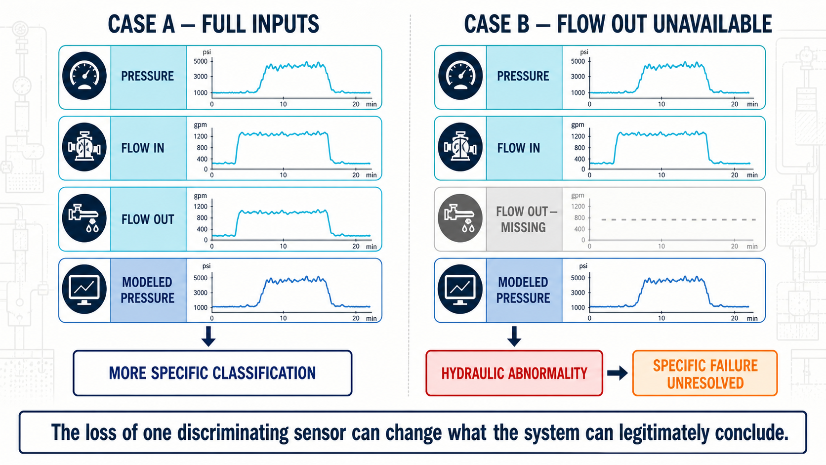
Loss of a discriminating sensor should reduce diagnostic specificity rather than leave confidence unchanged.

Practical Example: Torque and Drag

Suppose a tripping model normally evaluates:

• hook-load deviation,
• hook-load trend,
• friction factor,
• tripping direction.

Now hook load disappears.

The system may still know:

• tripping direction,
• some contextual friction expectation.

But one of the strongest mechanical observations is missing.

A robust model lowers the influence of that feature rather than fabricating a trend.

The user should similarly see:

Overpull assessment degraded because hook-load data is unavailable.

This turns degraded analytics into useful data-quality information.

When Should a System Abstain?

A practical framework might consider several reasons.

Required sensor missing

The model cannot evaluate a key discriminating signal.

Context unresolved

Examples:

• wrong BHA,
• unknown wellbore,
• formation unavailable.

Model outside validated domain

The current operating state falls outside the model's intended conditions.

Competing explanations remain indistinguishable

Several causes fit the evidence almost equally well.

Evidence conflicts materially

Sources or signals point in contradictory directions.

Data quality is inadequate

Sensor confidence is too low.

Sample history is insufficient

Trend calculations do not yet have enough data.

Any of these can justify:

Unable to Determine

or a deliberately broader conclusion.

Unknown Should Be Treated as a First-Class Data Product

This is an architectural point.

Do not encode unknown as:

• zero,
• null without meaning,
• normal,
• other.

Instead, preserve explicit state.

For example:

$$status = \text{INSUFFICIENT\_EVIDENCE}$$

with fields such as:

• reason,
• missing inputs,
• affected calculations,
• timestamp,
• suggested next evidence.

Then downstream dashboards and AI systems can treat uncertainty correctly.

A Practical Output Schema

Conceptually, an engineering event could contain:

• event_family: hydraulic abnormality
• specific_diagnosis: unresolved
• confidence_in_family: high
• confidence_in_specific_cause: insufficient
• missing_evidence: flow out
• observed_evidence: pressure-model deviation
• next_check: verify pump/flow behavior

The important design principle is separation.

Confidence in:

something is wrong

does not have to equal confidence in:

exactly what is wrong.

DrillingMetrics / AIDE Screenshot Opportunity

This article would benefit most from a real example where the interface exposes missing or conflicting evidence.

A good DrillingMetrics figure could show:

• synchronized pressure/flow signals,
• one unavailable channel,
• model-versus-measurement comparison.

If the product does not currently expose an explicit unknown state, do not manufacture one.

For AIDE, an even stronger example would be a real response where the assistant says that a question cannot be answered conclusively from the available data and explains what information is missing.

That would demonstrate an unusually important product behavior:

the ability to resist producing a confident answer merely because the interface is conversational.

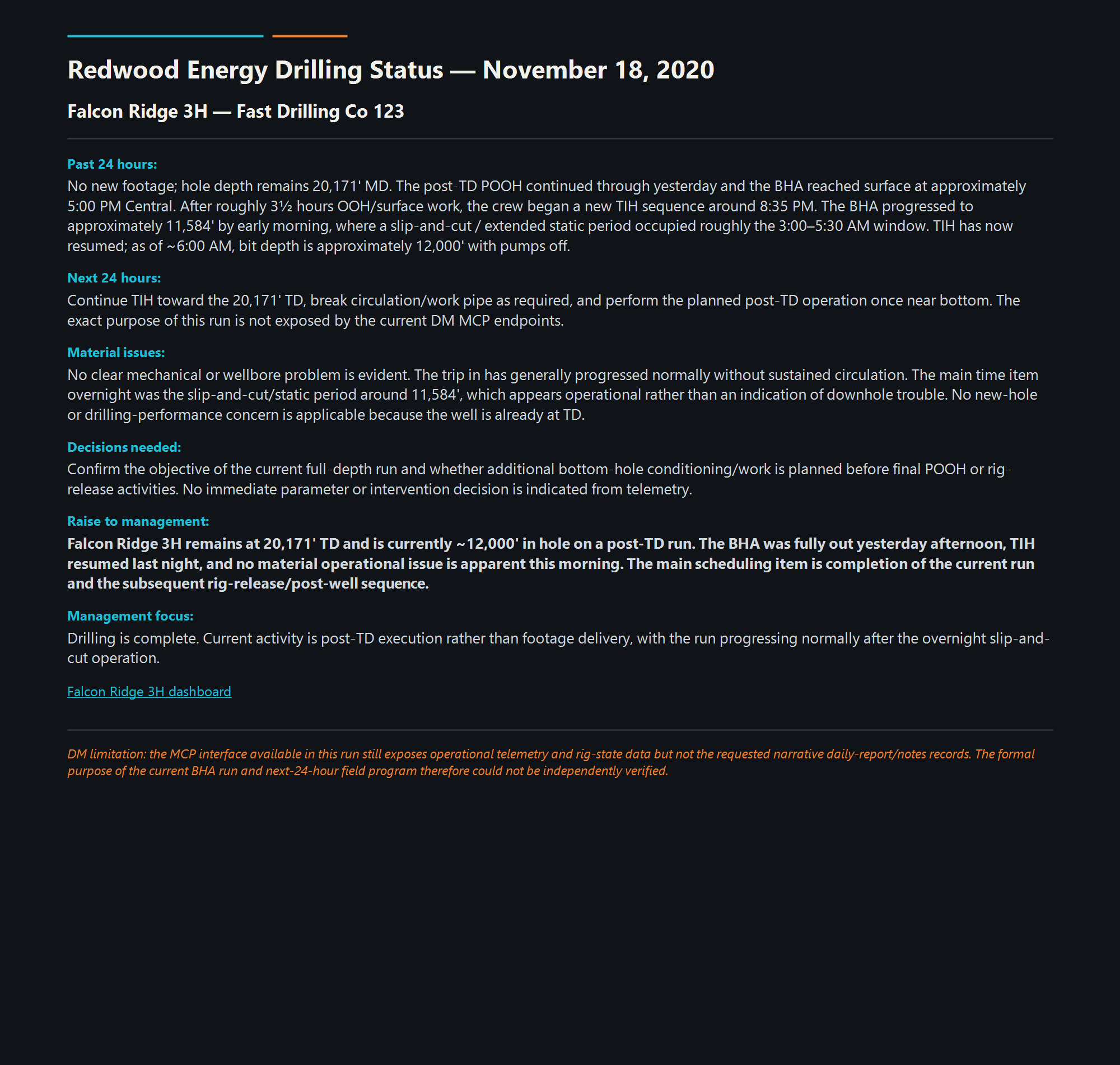
This schedule-MCP status reports what telemetry supports and states that the run objective could not be verified because daily-report and notes context was unavailable.

A Reliability Hierarchy

A useful engineering intelligence system should prefer:

1. Correct specific answer

when evidence supports it.

2. Correct broad answer

when evidence supports only the broader class.

3. Explicit uncertainty

when competing explanations remain.

4. Unable to determine

when evidence is insufficient.

What it should avoid is:

5. Specific but unsupported answer

That last output may appear the most intelligent.

It is often the least reliable.

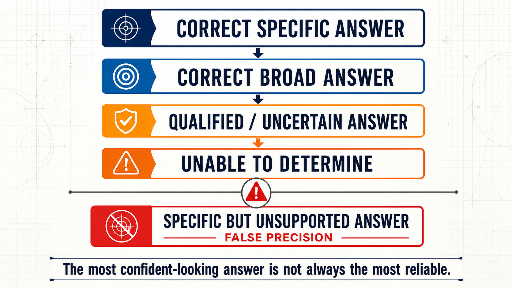
Reliable engineering intelligence prefers a correct broad or uncertain answer over unsupported specificity.

The Goal Is Calibrated Specificity

This article is not an argument for analytical systems to become timid.

A useful system should still detect:

• strong patterns,
• meaningful changes,
• high-confidence failures.

The objective is:

match the specificity of the conclusion to the strength of the evidence.

When the evidence becomes stronger:

be more specific.

When it becomes weaker:

broaden the conclusion.

When it becomes inadequate:

say so.

That is calibrated engineering reasoning.

Conclusion

Drilling analytics operates in a world of incomplete information.

Sensors fail.

Models are approximate.

Context can be stale.

Several physical events can create similar surface signatures.

It is therefore unrealistic to expect every analytical question to have a unique answer at every instant.

A system that always returns a diagnosis does not eliminate uncertainty.

It hides it.

A more trustworthy system represents uncertainty explicitly.

Sometimes the correct output is:

Normal.

Sometimes:

Fault likely.

Sometimes:

Hydraulic abnormality detected; specific cause unresolved.

And sometimes:

Unable to determine from the available evidence.

That final output should not be viewed as an analytical failure.

It can be one of the clearest signs that the system understands what its data actually supports.

In drilling engineering, confidence should come from evidence—not from the software's willingness to produce an answer.

---

References

1. Ashok, P., Ambrus, A., Ramos, D., Lutteringer, J., Behounek, M., Yang, Y. L., Thetford, T., and Weaver, T. A Step by Step Approach to Improving Data Quality in Drilling Operations: Field Trials in North America. SPE-181076-MS, SPE Intelligent Energy International Conference and Exhibition, Aberdeen, Scotland, 2016.

2. Ambrus, A., Ashok, P., Thetford, T., Behounek, M., and others. Drillstring Washout and Mud Pump Failure Detection Using Real-Time Data and Physics-Based Modeling. IADC/SPE-189700-MS, 2018.

3. Shahri, M., Wilson, T., Thetford, T., Nelson, B., Behounek, M., Ambrus, A., D'Angelo, J., and Ashok, P. Implementation of a Fully Automated Real-Time Torque and Drag Model for Improving Drilling Performance: Case Study. SPE-191426-MS, SPE Annual Technical Conference and Exhibition, Dallas, Texas, 2018.

4. Behounek, M., Thetford, T., Yang, L., Hofer, E., White, M., Ashok, P., Ambrus, A., and Ramos, D. Human Factors Engineering in the Design and Deployment of a Novel Data Aggregation and Distribution System for Drilling Operations. SPE/IADC-184743-MS, SPE/IADC Drilling Conference and Exhibition, The Hague, Netherlands, 2017.