Detecting Invisible Lost Time from Drilling Activity Data

The largest performance opportunities are not always recorded as NPT. Small, repeated delays in connections, transitions, trips, and routine workflows can accumulate into substantial well time.

When a drilling operation loses six hours to a failed mud pump, the lost time is obvious.

It is recorded.

It is discussed.

It may appear in a morning report, NPT tracker, or end-of-well review.

Now consider a different problem.

Every drilling connection on one rig takes 90 seconds longer than necessary.

There are 220 connections during the well.

The additional time is:

$$ 220 \times 90\text{ sec} = 19,800\text{ sec} $$

or:

$$ 5.5\text{ hours} $$

Nothing failed.

There may be no NPT entry.

No single connection looked alarming.

Yet the well still took more than five additional hours.

That is the nature of invisible lost time.

It often lives in the gap between:

what an operation must take

and

what it actually takes.

SPE/IADC-184743 describes invisible-lost-time analysis as a method for identifying workflow and process improvements on drilling rigs.[1]

The key word is process.

ILT is not necessarily an equipment failure.

It is frequently the accumulation of small, repeatable inefficiencies in otherwise normal operations.

And because those inefficiencies are repetitive, real-time rig-state data provides an unusually powerful way to find them.

Invisible lost time usually appears as small, repeated workflow inefficiencies rather than one obvious failure.

NPT and ILT Are Different Performance Problems

Nonproductive time is usually associated with a recognizable event:

• equipment failure,
• stuck pipe,
• lost circulation,
• waiting on materials,
• fishing,
• well-control problems.

The operation has departed from the planned workflow.

Invisible lost time is more subtle.

The rig may still be performing the intended operation.

It is simply performing it less efficiently than it reasonably could.

Examples might include:

• slow drilling connections,
• delayed transitions back to bottom,
• excessive time preparing for a connection,
• inconsistent tripping connections,
• unnecessarily long pump-start procedures,
• repeated short delays between otherwise normal states.

The distinction matters because the improvement method is different.

For NPT, the question may be:

How do we prevent this failure from happening again?

For ILT, the question is more often:

Why does this routine operation consistently take longer than our demonstrated best performance?

That is a benchmarking problem.

One Slow Event Usually Does Not Matter

Suppose a drilling connection takes 7.5 minutes.

Is that bad?

Not necessarily.

There may have been:

• a required operational check,
• an unusual pressure response,
• crew coordination,
• a temporary equipment constraint.

One observation rarely tells us much.

Now suppose we examine 180 connections.

The distribution looks like this:

• P10: 4.2 min
• P25: 4.6 min
• median: 5.1 min
• P75: 5.9 min
• P90: 7.3 min

Now the question becomes more interesting.

The rig has repeatedly demonstrated that the operation can be completed in roughly 4–5 minutes.

But a substantial fraction of events take much longer.

That creates an identifiable performance opportunity.

This is why ILT analysis is fundamentally statistical.

The objective should not be to find the single fastest event and declare every other event inefficient.

The objective is to understand the distribution.

A repeatable percentile is often a more defensible operational benchmark than the single fastest event.

The Fastest Event Is Usually the Wrong Benchmark

It is tempting to say:

Our fastest connection was 3.8 minutes, so every connection should take 3.8 minutes.

That is usually too aggressive.

The fastest observation may have benefited from:

• favorable sequencing,
• unusually simple conditions,
• measurement noise,
• incomplete event boundaries,
• or circumstances that are not repeatable.

A more useful benchmark is often based on a percentile.

For example:

P25 connection time

can represent performance that has already been demonstrated regularly—not merely once.

If the rig's P25 is 4.6 minutes and its median is 5.1 minutes, improving the median toward the lower quartile may be a realistic initial target.

The target comes from demonstrated operational capability.

Not from an arbitrary number.

This is one reason percentile-based benchmarking is often more useful than comparing averages alone.

Average Time Can Hide the Shape of the Problem

Consider two rigs.

Rig A

Connection times:

• tightly clustered around 5.5 minutes.

Rig B

Most connections:

• around 4.5 minutes,

but a minority:

• 9–12 minutes.

Both rigs might have an average around 5.5 minutes.

Operationally, they have very different problems.

Rig A appears consistently slower.

The improvement opportunity may involve the normal workflow itself.

Rig B appears capable of faster routine execution, but has intermittent events creating a long tail.

The investigation should therefore focus on:

What is different about the slow events?

That might involve:

• specific crews,
• specific depths,
• particular equipment conditions,
• shift changes,
• pump behavior,
• particular hole sections,
• or another recurring operational pattern.

Averages erase much of this information.

Distributions preserve it.

Two rigs with the same average connection time can require completely different improvement strategies.

Rig State Creates the Event Boundaries

Before a connection can be timed automatically, the system has to identify when it begins and ends.

That requires operational-state information.

Conceptually, a drilling connection may look like:

Drilling

↓

Come Off Bottom

↓

Connection Activity

↓

Return Toward Bottom

↓

Drilling Resumes

Each transition creates a timestamp.

From those timestamps, different pieces of the workflow can be measured.

For example:

Pre-connection transition

How long does it take from leaving the drilling condition to beginning the actual connection activity?

Connection activity

How long does the pipe-handling / slips portion take?

Post-connection transition

How long does it take after the connection is completed to return to drilling?

Complete cycle

How much time passes between the end of one drilling interval and the beginning of the next?

The exact KPI names are less important than the principle:

Do not reduce the workflow to one number if the objective is to improve the workflow.

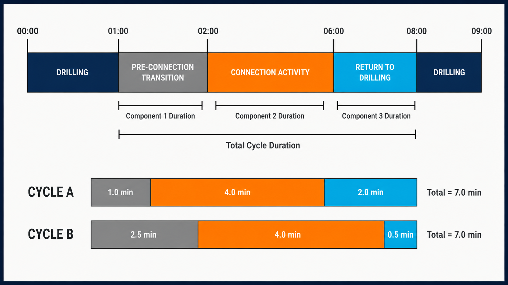
Segmenting a routine connection into operational phases identifies where the additional time actually occurs.

A Slow Connection Is Not Necessarily a Slow Connection Operation

This is where segmentation becomes valuable.

Suppose two connection cycles both take seven minutes.

Event A

• pre-connection: 1.0 min
• connection: 4.0 min
• return to drilling: 2.0 min

Event B

• pre-connection: 2.5 min
• connection: 4.0 min
• return to drilling: 0.5 min

The total time is identical.

But the improvement opportunity is not.

The crew performs the central connection activity equally fast in both events.

Event A loses time after the connection.

Event B loses time before it.

If only total connection time is tracked, these two workflows look the same.

They are not.

This is the broader lesson:

Performance KPIs should preserve enough process structure to remain actionable.

ILT Is the Difference Between Actual and Achievable Performance

A useful conceptual definition is:

$$ ILT_i = T_{actual,i} - T_{benchmark,i} $$

for event i, when:

$$ T_{actual,i} > T_{benchmark,i} $$

Suppose:

• benchmark connection cycle = 4.8 min
• actual connection = 6.0 min

Then the opportunity is:

$$ ILT = 1.2\text{ min} $$

Do that 150 times:

$$ 150 \times 1.2 = 180\text{ min} $$

or:

3 hours.

This simple calculation illustrates why individually small improvements matter.

But the benchmark has to be defensible.

It should ideally account for differences in:

• operation type,
• rig,
• hole section,
• depth,
• equipment configuration,
• and other relevant context.

Comparing unlike operations can manufacture ILT that does not actually exist.

Benchmark the Same Process Against the Same Process

Suppose one rig's connection performance in surface hole is compared directly with another rig's lateral performance.

Is that fair?

Maybe not.

Operational conditions can change with:

• pipe size,
• stand configuration,
• rig equipment,
• depth,
• pump procedures,
• hole section,
• mud system,
• crew practices.

Likewise, tripping connections should not automatically be pooled with drilling connections.

The correct population depends on the question.

A defensible workflow is:

1. classify the operation,
2. define comparable events,
3. normalize relevant context,
4. then compare performance.

This is the same analytical principle that appears throughout drilling performance analysis:

Benchmarking requires comparable populations.

Crew Comparison Requires Particular Care

ILT data makes crew comparisons easy.

That does not automatically make them fair.

Suppose Day Crew has median connection time:

4.8 min

and Night Crew:

5.5 min

It is tempting to conclude that the day crew is better.

But first ask:

• Were they operating in comparable hole sections?
• Were equipment conditions the same?
• Did one shift encounter more troubleshooting?
• Was one crew performing more unusual procedures?
• Is the sample size large enough?
• Are connection boundaries classified consistently?

Crew comparison becomes meaningful only after context has been controlled sufficiently.

The goal of ILT analysis should be process improvement—not producing simplistic rankings from heterogeneous data.

Depth Can Reveal Where Time Is Being Lost

Time distributions tell us how much operations vary.

Depth tells us where the variation occurs.

SPE/IADC-184743 describes a high-resolution days-versus-depth approach using real-time data rather than one daily point. The purpose was to expose flat spots that conventional daily plots could hide and allow engineers to investigate what occurred at those depths.[1]

That concept is extremely useful for ILT.

Imagine a depth plot where the well progresses steadily for several thousand feet.

Then around 11,800–12,300 ft:

the curve becomes noticeably flatter.

There may be no formal NPT event.

But that interval consumed more clock time per foot.

The next question becomes:

Which rig states occupied the additional time?

Perhaps:

• more reaming,
• slower connections,
• additional circulation,
• repeated downlinks,
• extra surveys,
• more slide drilling,
• reduced ROP.

The days-versus-depth plot identifies the location.

Rig-state analysis identifies the cause.

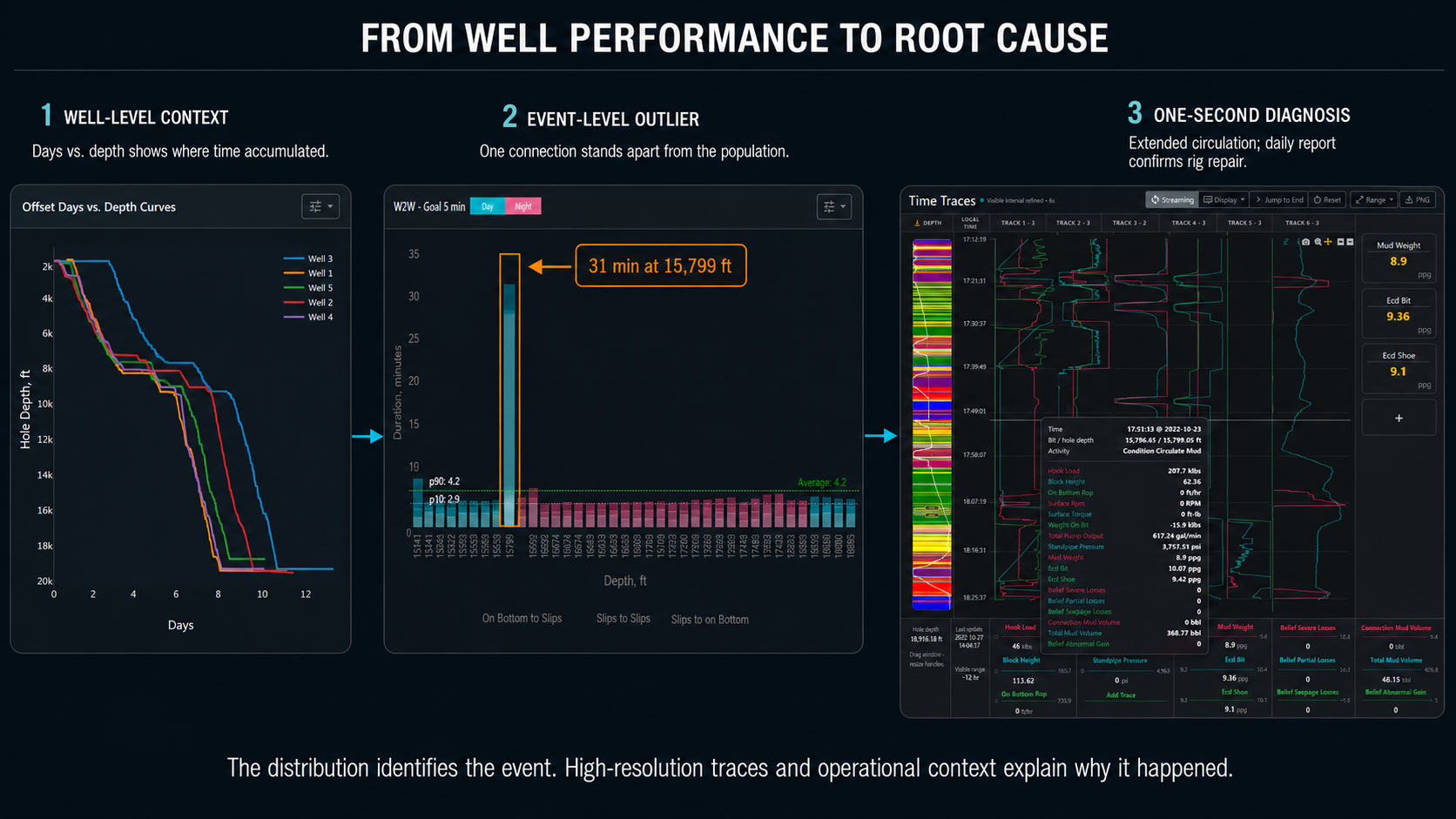
High-resolution days-versus-depth analysis locates where time accumulated; rig-state data explains which operations produced it.

Time Lost Per Event and Total Opportunity Are Different

Suppose two workflow opportunities are identified.

Operation A

• 30 seconds opportunity per event
• 250 occurrences

Total:

$$ 125\text{ min} $$

Operation B

• 5 minutes opportunity per event
• 10 occurrences

Total:

$$ 50\text{ min} $$

Operation B looks much worse when individual events are inspected.

Operation A has the larger effect on the well.

This suggests a useful prioritization quantity:

$$ Total\ Opportunity = Opportunity\ per\ Event \times Event\ Frequency $$

Small delays can dominate total well impact when they occur frequently.

The largest ILT opportunities are often not the worst-looking individual events.

They are the routine inefficiencies repeated most often.

This is why connections receive so much attention in drilling-performance analysis.

They happen hundreds of times.

Variability Is Itself a Performance Signal

Suppose a rig has median connection time of 5.0 minutes.

Is that good?

The answer becomes more useful when variability is included.

Rig A

• P25 = 4.8
• median = 5.0
• P75 = 5.3

Rig B

• P25 = 4.0
• median = 5.0
• P75 = 7.0

The medians are identical.

Rig A is highly repeatable.

Rig B occasionally performs much faster but is inconsistent.

This suggests two different improvement strategies.

For Rig A:

the process may already be controlled, and future gains may require redesigning the normal workflow.

For Rig B:

the fast process already exists.

The priority may be understanding why it is not repeated consistently.

That makes spread metrics such as:

$$ IQR = P75 - P25 $$

operationally useful.

ILT is not only about reducing the center of a distribution.

It can also mean reducing its variability.

Variation around the median reveals whether improvement requires a faster process or a more repeatable process.

The Slow Tail Deserves Investigation, Not Automatic Removal

Data analysts often remove outliers.

That can be dangerous in operational-performance analysis.

Suppose connection times above 10 minutes are classified as statistical outliers and removed.

Those may be exactly the events the drilling engineer needs to investigate.

An outlier might represent:

• equipment hesitation,
• manual intervention,
• procedural inconsistency,
• a repeated sensor/classification issue,
• or a real operational constraint.

Cleaning the distribution by deleting those observations can hide the improvement opportunity.

The better workflow is:

classify first, investigate second, exclude only with a reason.

For example:

A connection involving a documented equipment repair may legitimately belong outside routine connection benchmarking.

A connection that simply took 11 minutes for no identified reason may be ILT.

Statistical abnormality alone does not determine which.

Necessary Time Should Not Be Called Lost Time

This point is important.

Not all flat time is bad.

Operations may intentionally require:

• circulating,
• flow checks,
• surveys,
• downlinks,
• well-control precautions,
• hole conditioning,
• equipment inspections.

If those actions reduce operational risk, the correct objective is not necessarily to eliminate them.

ILT analysis should distinguish:

required process time

from

avoidable excess time.

For example, if a connection includes a mandatory 60-second flow check, benchmarking the operation against a rig that does not perform that check is misleading.

The benchmark should reflect the workflow actually required.

The goal is not:

Minimize every non-drilling second.

It is:

Execute necessary operations consistently and efficiently while identifying delays that add no corresponding operational value.

Faster Is Not Always Better

Suppose one crew reduces connection time by aggressively accelerating every transition.

Total well time improves.

But suppose the change also creates:

• repeated pressure transients,
• poor hole cleaning,
• equipment damage,
• unsafe pipe-handling behavior.

That is not optimization.

Performance metrics should operate within engineering and safety constraints.

A useful formulation is:

$$ Minimize\ Routine\ Time $$

subject to:

$$ Safety,\ Equipment,\ Wellbore,\ and\ Operational\ Constraints $$

This is why ILT should be treated as process engineering, not a race.

ILT Can Appear While Drilling Too

The concept is not limited to connections.

Consider two rotary-drilling intervals in the same formation.

Both are classified as productive drilling.

One averages:

180 ft/hr

The other:

140 ft/hr

No dysfunction is formally recorded.

No NPT occurs.

The second interval still consumes more time per foot.

Some of that difference may be unavoidable geology.

Some may reflect:

• poorer parameter selection,
• inefficient drilling mechanics,
• changing bit condition,
• less effective hydraulics.

This means invisible lost time can exist inside a nominally productive state.

The analysis simply becomes more complicated because geology and equipment condition must be normalized.

That is where the earlier ROP/MSE articles connect to ILT.

Workflow ILT and drilling-efficiency ILT are related but analytically different problems.

A Practical Connection Example

Consider a hypothetical well containing 200 drilling connections.

The connection-cycle distribution is:

• P25 = 4.5 min
• median = 5.2 min
• P75 = 6.0 min
• P90 = 7.4 min

Rather than using the single fastest connection, management chooses:

4.7 minutes

as a realistic benchmark based on consistently demonstrated performance.

The average excess above that benchmark across the 200 connections is:

0.8 minutes/event.

Total opportunity:

$$ 200 \times 0.8 = 160\text{ minutes} $$

or about:

2.7 hours.

Now segment the slow events.

The additional time comes from:

• pre-connection: 15%
• central connection activity: 20%
• return-to-drilling transition: 65%

That changes the operational recommendation completely.

The main opportunity is not:

make connections faster.

It is:

reduce the delay between completion of the connection and resumption of productive drilling.

That is what actionable ILT analysis should do.

A 31-minute connection stands outside the surrounding population. One-second traces show extended circulation; daily reporting confirmed that the delay coincided with a rig repair.

Comparing Wells Requires Standard KPI Definitions

SPE/IADC-184743 makes a valuable point about ILT reporting: different users may prefer different KPIs, but standardized comparisons are still necessary so engineers discussing improvement are evaluating the same thing.[1]

That sounds administrative.

It is actually a data-engineering requirement.

Suppose Team A defines a connection from:

bit off bottom → drilling resumes

while Team B defines it from:

slips engaged → slips released.

Both report:

Connection Time

Their numbers are not comparable.

Standardization therefore requires agreement on:

• event start,
• event end,
• states included,
• treatment of interruptions,
• treatment of invalid data,
• minimum/maximum valid event duration,
• handling of partial events,
• depth attribution.

Without those definitions, a fleet-wide KPI dashboard may compare different processes under identical labels.

State-Classifier Changes Can Change Historical KPIs

There is another subtle issue.

Suppose the rig-state classifier is improved.

Some intervals previously labeled:

Connection

are now correctly identified as:

Circulation

Historical connection statistics change.

Did operational performance change?

No.

The measurement system changed.

This is conceptually similar to the survey-resolution issue in tortuosity analysis.

A KPI is influenced by:

1. the underlying physical operation,
2. the method used to classify and calculate it.

Therefore, automated ILT systems should ideally preserve:

• classifier version,
• KPI-definition version,
• processing history.

If the definition changes, historical comparisons should be recalculated consistently or clearly identified as using different methodologies.

Good ILT Reporting Prioritizes Decisions

A report containing 40 charts can technically contain more information than a report containing five.

It may also be less useful.

SPE/IADC-184743 specifically notes that ILT reports can become unwieldy when they contain too many plots and emphasizes customizable reporting while retaining standardized comparisons.[1]

A useful ILT report might therefore answer only a few questions:

1. Where was the largest total time opportunity?
2. Which routine operation generated it?
3. Was the issue slower typical performance or high variability?
4. At which depths, crews, or shifts was it concentrated?
5. What benchmark has already been demonstrated repeatedly?

Everything else can remain available for investigation.

The summary should direct attention.

The detailed data should provide evidence.

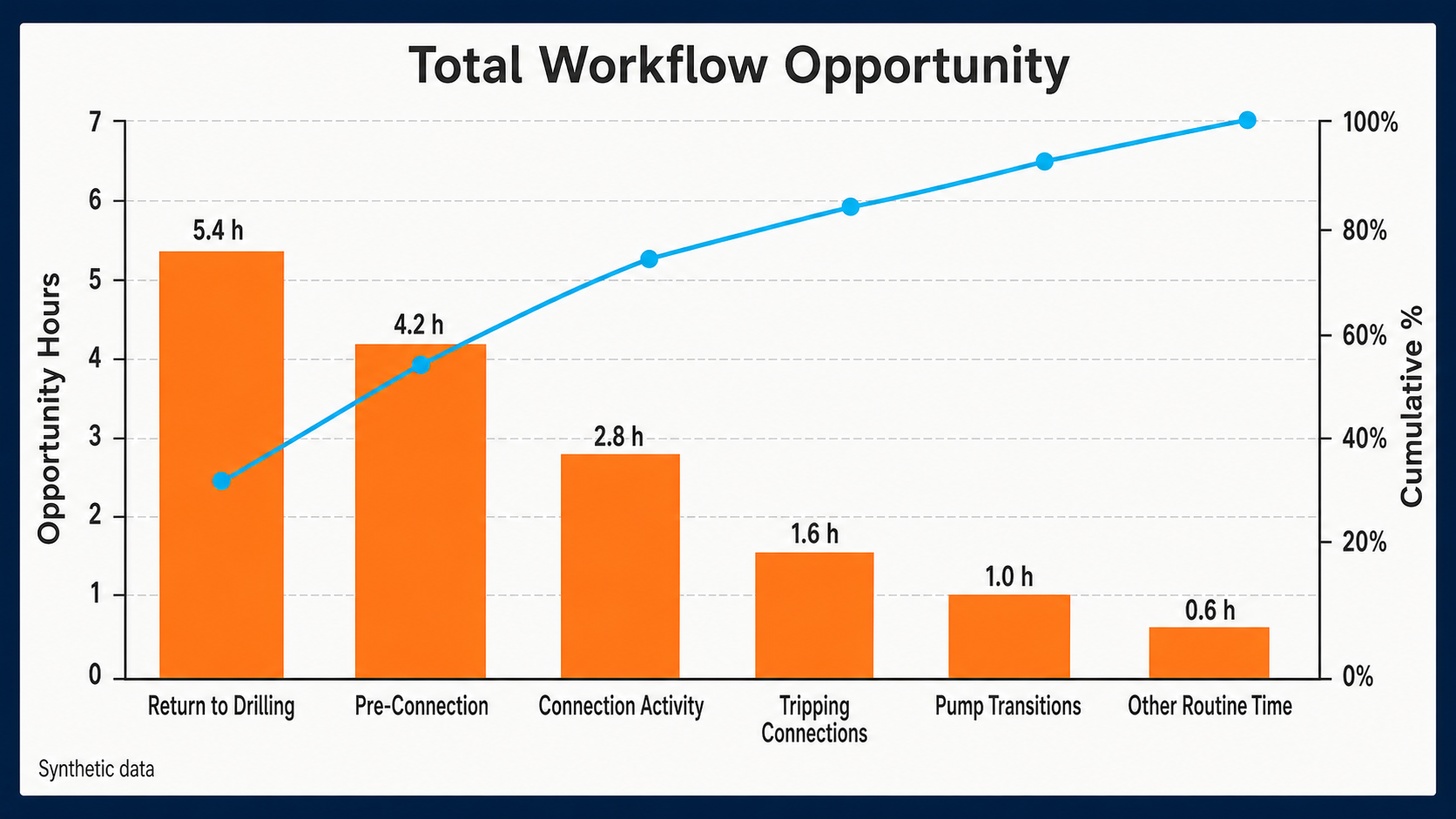
Ranking total opportunity rather than individual-event severity focuses improvement on the workflows that matter most to overall well time.

From Measuring Time to Improving a Process

A mature ILT workflow should not end with:

Rig A loses 3.2 hours per well in connections.

That is only a diagnosis.

The next step is understanding why.

A useful improvement loop is:

1. Detect states

Convert raw rig channels into operational activity.

2. Segment events

Identify repeatable workflow cycles.

3. Calculate distributions

Measure:

• median,
• percentiles,
• variability,
• event counts.

4. Establish a realistic benchmark

Use repeatable demonstrated performance rather than an isolated record.

5. Quantify total opportunity

Combine excess time per event with frequency.

6. Localize the opportunity

Break the event into operational phases.

7. Search for explanatory context

Compare:

• crew,
• shift,
• depth,
• rig,
• equipment,
• hole section,
• procedure.

8. Change the workflow

Implement a specific operational improvement.

9. Measure again

Determine whether the distribution actually shifted.

That final step is essential.

Without it, ILT analysis becomes another report.

With it, ILT becomes a continuous-improvement system.

ILT analytics creates value when measurement leads to a workflow change and the operation is measured again.

The Goal Is Not the Record Connection

A drilling team can always focus on a record:

Fastest connection: 3.6 minutes

That may be motivating.

It is not necessarily operationally important.

Consider a rig with:

• fastest = 3.6 min
• median = 6.0 min.

Now consider another:

• fastest = 4.1 min
• median = 4.5 min.

The second rig may produce substantially less total flat time despite never setting the record.

This is why high-performance drilling is often more about repeatability than isolated excellence.

A good ILT program attempts to move the entire distribution.

Not merely its best point.

Invisible Lost Time Becomes Visible When Routine Work Is Structured as Data

The fundamental insight is straightforward.

The drilling operation already contains the information required to understand much of its workflow performance.

Every cycle leaves evidence in:

• bit depth,
• hole depth,
• block movement,
• hook load,
• pumps,
• RPM,
• and operational state.

Rig-state classification turns those signals into events.

Event segmentation turns events into durations.

Statistics turn durations into performance distributions.

Benchmarking turns distributions into measurable opportunities.

And repeated analysis turns those opportunities into process improvement.

That progression is what makes ILT measurable:

$$ Sensors \rightarrow States \rightarrow Events \rightarrow KPIs \rightarrow Distributions \rightarrow Opportunity \rightarrow Improvement $$

The time was always there.

The difference is that now the operation has enough structure to see it.

---

References

1. Behounek, M., Thetford, T., Yang, L., Hofer, E., White, M., Ashok, P., Ambrus, A., and Ramos, D. Human Factors Engineering in the Design and Deployment of a Novel Data Aggregation and Distribution System for Drilling Operations. SPE/IADC-184743-MS, SPE/IADC Drilling Conference and Exhibition, The Hague, Netherlands, 2017.

2. Shahri, M., Wilson, T., Thetford, T., Nelson, B., Behounek, M., Ambrus, A., D'Angelo, J., and Ashok, P. Implementation of a Fully Automated Real-Time Torque and Drag Model for Improving Drilling Performance: Case Study. SPE-191426-MS, SPE Annual Technical Conference and Exhibition, Dallas, Texas, 2018.