The Nonlinear WOB–RPM Performance Landscape

Drilling performance does not usually improve smoothly as WOB or RPM increases. Efficient operating regions can shift, split, disappear, and change as formation, bit condition, BHA behavior, hole condition, and dysfunction evolve.

Imagine plotting every rotary-drilling observation from a lateral on a simple two-dimensional chart.

Horizontal axis:

RPM

Vertical axis:

WOB

Color each point by ROP.

The intuitive expectation might be:

• low WOB and low RPM → poor performance,
• increase both → ROP improves,
• eventually reach an optimum,
• move beyond it → performance declines.

In other words, we might expect one smooth hill.

Find the top of the hill.

Operate there.

Real drilling frequently looks nothing like that.

Instead, the landscape may contain:

• several strong operating regions,
• low-performance pockets,
• narrow dysfunction zones,
• broad areas with similar ROP,
• gaps where little historical data exists,
• and operating regions that move as the well changes.

SPE-186166 provides a useful field example. Six wells from the same pad were selected specifically to create a relatively uniform comparison, and the data was filtered to rotary drilling.[1]

Even then, the authors found that drilling parameters that worked well on one well could not reasonably be assumed optimal for another.

At one lateral depth, two wells operating at very similar WOB and RPM showed dramatically different calculated drilling efficiency.

Possible reasons included:

• bit condition,
• wellbore tortuosity,
• hole cleaning,
• mud-motor condition.

When the field data was expanded into WOB–RPM performance maps, the resulting operating landscape was described as highly nonlinear and non-convex.[1]

That is an important phrase.

It means drilling optimization is usually not:

Turn WOB and RPM toward one universal optimum.

It is closer to:

Find a good operating region for the drilling system that exists right now, remain inside mechanical and operational constraints, and keep reevaluating as the system changes.

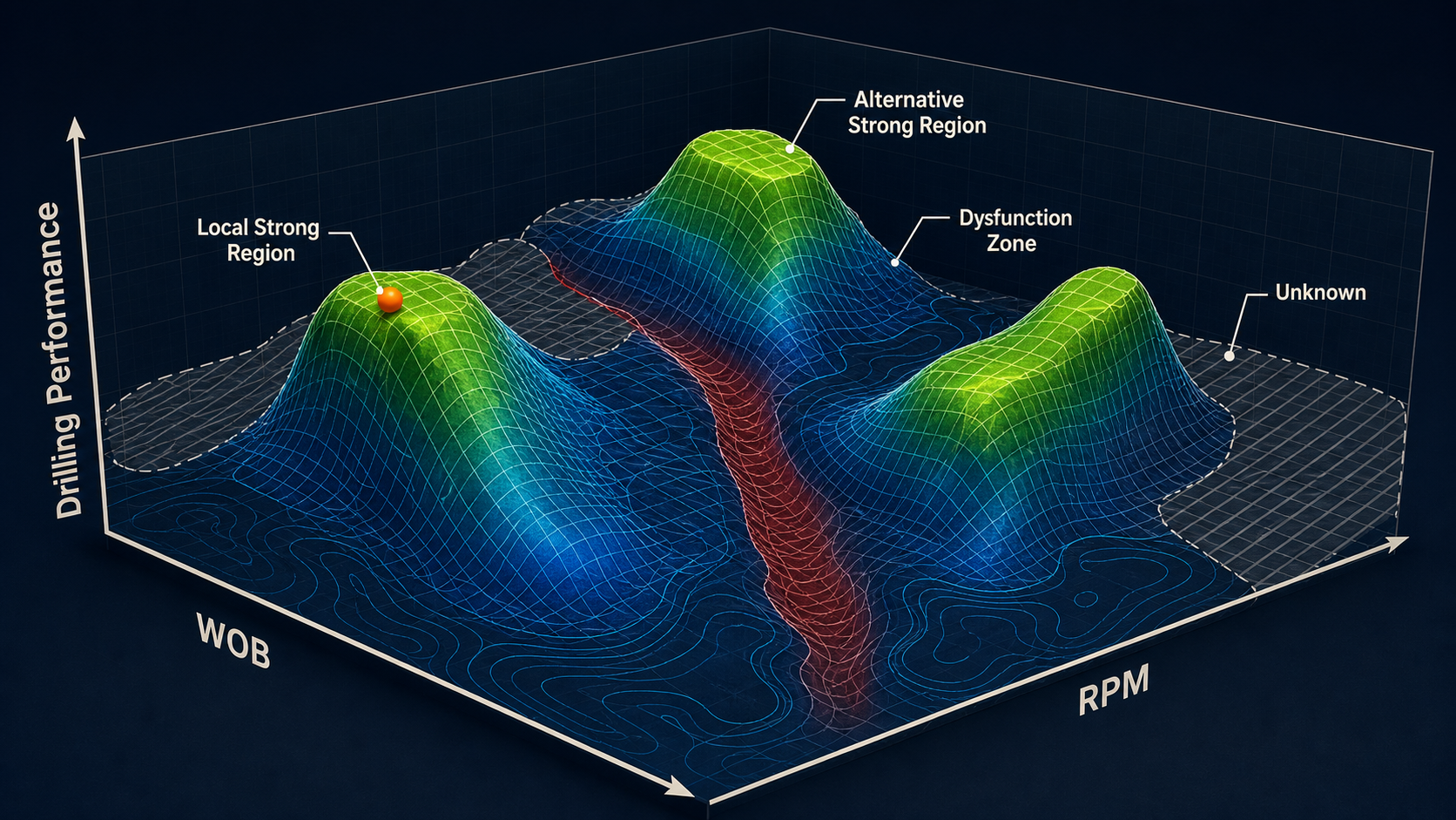
A nonlinear WOB–RPM landscape can contain several strong operating regions separated by valleys, dysfunction, and unexplored space.

What Does Nonlinear Actually Mean?

Suppose the current operating point is:

• WOB = 30 klbf
• RPM = 110
• ROP = 180 ft/hr.

Increase WOB to:

35 klbf

and ROP rises to:

215 ft/hr.

Increase again to:

40 klbf

and perhaps ROP rises only to:

220 ft/hr.

Increase to:

45 klbf

and torsional dysfunction develops.

ROP drops to:

170 ft/hr.

The response is not proportional.

Five additional klbf produced:

+35 ft/hr

in the first step,

+5 ft/hr

in the second,

and then:

−50 ft/hr

in the third.

That is nonlinear behavior.

The effect of changing WOB depends on where the system already is.

Likewise, the effect of changing RPM depends on:

• current WOB,
• formation,
• bit,
• BHA,
• dysfunction state.

A more realistic conceptual relationship is therefore:

$$Performance = f(WOB,RPM)$$

where $$f$$ is not a simple straight plane.

And even that is incomplete.

A better description is:

$$Performance = f( WOB, RPM \mid Formation, Bit, BHA, Hole\ Condition, Hydraulics, Dynamics, ... )$$

The vertical bar can be read as:

given the current drilling context.

Why a Smooth Surface Is So Appealing

Engineers naturally like maps.

A WOB–RPM heat map can turn thousands or millions of sensor observations into something intuitive.

For example:

• green = efficient,
• yellow = intermediate,
• red = poor.

The driller can see:

Current operating point

and:

better historical region

on the same screen.

That is extremely useful.

But the smooth appearance of the map can create a dangerous illusion:

continuous knowledge.

Field data is not continuous.

It consists of discrete operating points.

Suppose the historical wells mostly operated around:

• 25–30 klbf / 100–120 RPM,
• 35–40 klbf / 130–145 RPM.

There may be almost no observations around:

• 32 klbf / 125 RPM.

A contouring algorithm can still color that region.

Mathematically, it interpolates between nearby observations.

But the rig never actually demonstrated that exact operating condition.

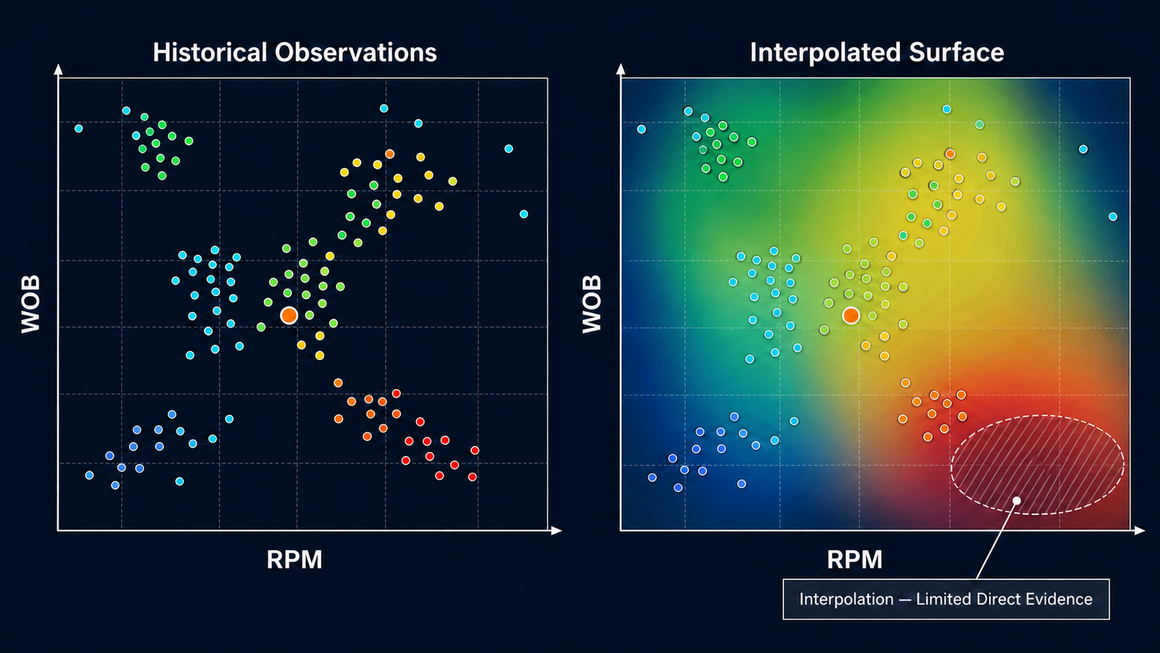
A smooth surface can imply more continuity and certainty than the underlying field observations support.

The Data Density Should Be Visible

A performance map should ideally answer two questions at the same time:

1. What performance was observed here?
2. How much evidence supports that conclusion?

Imagine two green areas.

Region A

Contains:

1,500 historical observations

from many stands and several wells.

Region B

Contains:

three observations

from one short interval.

A color map may display both as equally green.

They should not carry equal confidence.

Useful supporting information can include:

• observation count,
• footage represented,
• number of wells,
• number of stands,
• spread or variance.

A performance surface without data-density information risks converting a sparse observation into an apparently robust operating recommendation.

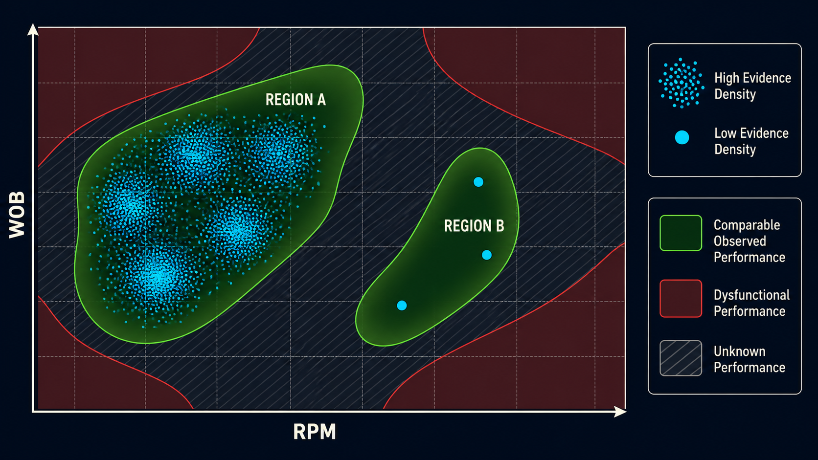
Comparable performance colors can carry very different levels of evidentiary support.

High ROP and High Efficiency Are Not the Same Surface

Another complication is the objective being mapped.

Suppose one heat map uses:

ROP

as the output.

Another uses:

MSE

or a broader drilling-efficiency index.

The maps may identify different preferred regions.

SPE-186166 presents field cases where wells experiencing lower calculated drilling efficiency still maintained relatively high ROP.[1]

That means:

$$\arg\max ROP$$

is not necessarily the same operating point as:

$$\arg\max Efficiency$$

or:

$$\arg\min MSE$$

This is important because the phrase:

optimal WOB and RPM

is meaningless until we define:

optimal for what?

Possible objectives include:

• maximum ROP,
• minimum MSE,
• minimum dysfunction,
• bit life,
• trajectory quality,
• total section time.

A WOB–RPM map reflects the objective used to color it.

One Parameter Change Can Improve One Metric and Hurt Another

Consider a hypothetical operating point.

Current:

• WOB = 35 klbf
• RPM = 100
• ROP = 210 ft/hr,
• moderate stick-slip.

Increase RPM to:

125.

Suppose:

• stick-slip improves,
• ROP rises to 225 ft/hr,
• torque oscillation decreases.

That looks clearly favorable.

Now increase RPM to:

155.

Suppose:

• ROP rises only slightly,
• vibration increases,
• bit wear risk increases.

The second move may still improve the ROP heat map.

It may worsen the broader drilling objective.

This is why parameter optimization should normally operate inside:

equipment + wellbore + dysfunction constraints.

Dysfunction Zones Can Split the Landscape

Stick-slip and whirl provide a useful example.

SPE-186166 found different portions of WOB–RPM space associated with different dysfunction behavior in its field data.[1]

That matters because the parameter response to one dysfunction may not be appropriate for another.

Conceptually, imagine:

Region A

High WOB
Low RPM

associated with torsional instability.

A move toward higher RPM may help.

Region B

Low WOB
Moderate/high RPM

associated with a different inefficient drilling mode.

Increasing RPM further may be the wrong direction.

Therefore, a rule such as:

MSE high → increase RPM

is incomplete.

The correct direction depends on where the current operating point lies relative to the type of dysfunction present.

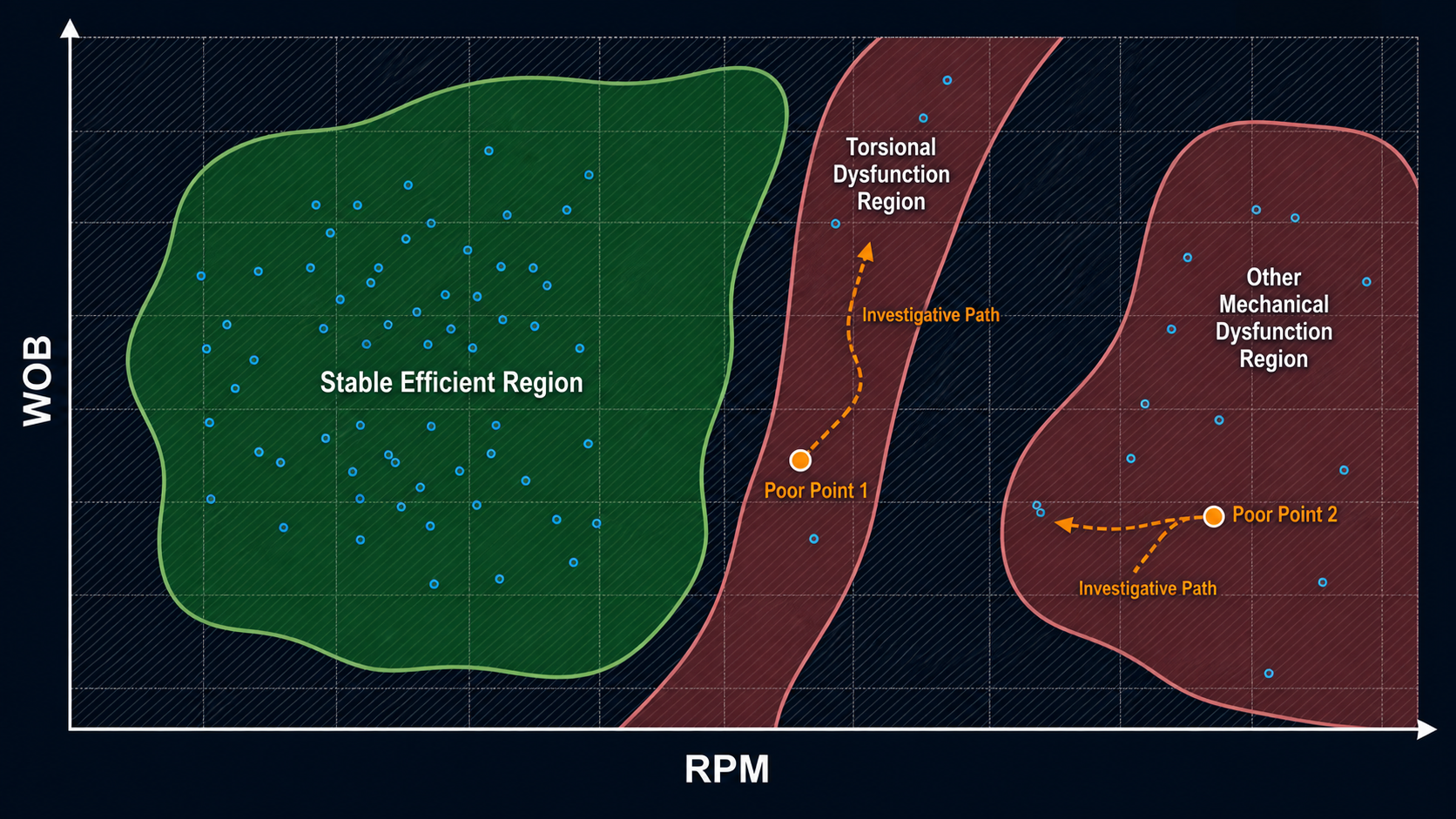
Different dysfunction neighborhoods can justify different investigative paths; no one parameter direction is universally correct.

Non-Convex Means Several "Better" Directions May Exist

A convex optimization landscape has a useful property.

If you move uphill locally, you eventually reach the single best point.

A non-convex landscape can contain:

• several peaks,
• ridges,
• valleys,
• local optima.

Imagine standing on one high-performing region.

There may be another region with better performance elsewhere.

But reaching it requires temporarily moving through worse performance.

Operationally, the driller cannot explore arbitrary parameter combinations simply to map the entire landscape.

The well is not a laboratory experiment with unlimited trials.

There are:

• equipment limits,
• dysfunction risk,
• formation changes,
• limited footage,
• time constraints.

So the real practical objective is often not:

find the mathematical global optimum.

It is:

find a strong, stable operating region safely and efficiently.

That is a different optimization problem.

The Well Changes While You Are Mapping It

There is another fundamental problem.

The performance landscape itself is not stationary.

Suppose the rig spends several hundred feet exploring WOB/RPM combinations.

By the time enough observations exist:

• formation may have changed,
• bit may be more worn,
• lateral may be longer,
• torque transfer may have changed,
• hole condition may have changed.

The map being learned is moving underneath the optimization process.

Formally, instead of:

$$Performance=f(WOB,RPM)$$

we really have something closer to:

$$Performance = f(WOB,RPM,Context_t)$$

where $$Context_t$$ changes with time and depth.

That is why historical maps should be treated as priors rather than permanent truth.

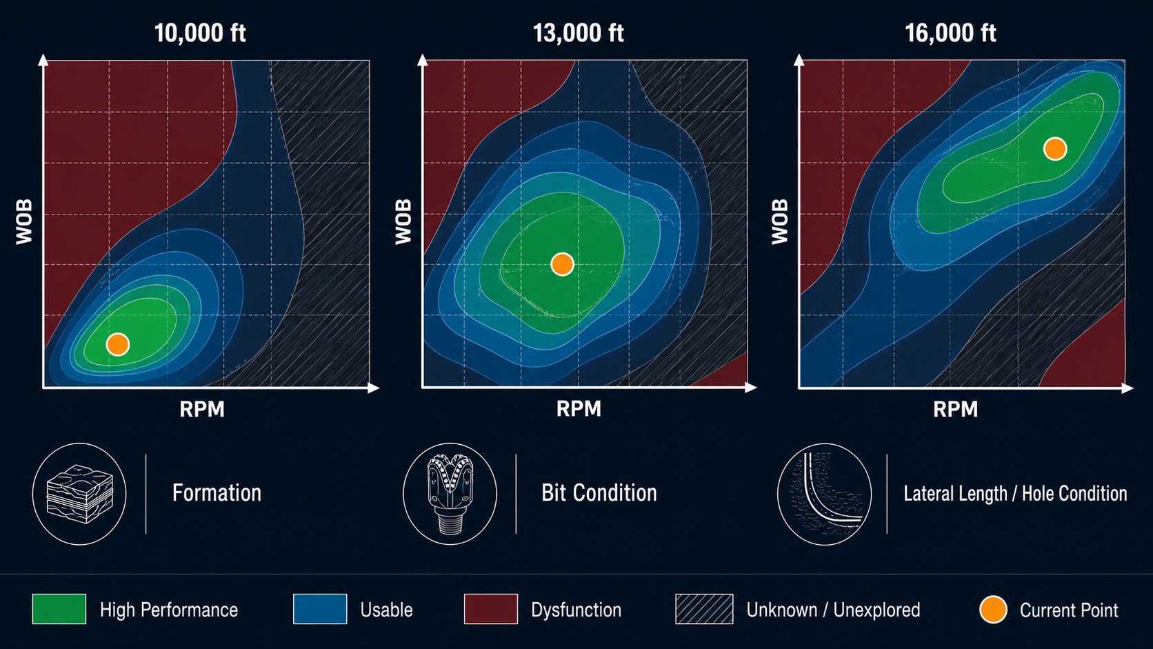
Formation, bit condition, and hole condition can move and reshape the strong operating region as depth increases.

Formation Can Move the Entire Landscape

Suppose the best operating region in Formation A is approximately:

• 35–40 klbf WOB,
• 120–140 RPM.

The well enters Formation B.

Rock strength changes.

The same operating point may now produce:

• lower ROP,
• higher MSE,
• different torque response.

The mathematical coordinates:

35 klbf / 130 RPM

have not changed.

The physical system has.

SPE-186166 explicitly separated performance maps by formation, and its conclusion emphasizes uncertainty from formation changes as one reason optimal regions differ.[1]

That is the correct way to think about WOB–RPM maps.

The axes are universal.

The response surface is contextual.

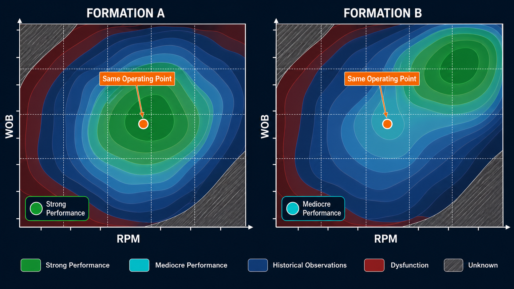
The same WOB–RPM point can perform differently after the formation—and therefore the response surface—changes.

Bit Condition Changes the Map Too

Now keep the formation constant.

At the beginning of a bit run:

• cutters are sharp,
• ROP responds strongly to increased WOB.

Later:

• bit condition deteriorates,
• additional WOB produces less ROP,
• torque may increase.

The WOB–RPM landscape has changed again.

An operating region that was efficient 4,000 ft ago may no longer be efficient.

This is one reason historical parameter recipes should not be treated as static throughout a long lateral.

Hole Condition Is Another Hidden Axis

Suppose two wells use:

• the same bit,
• the same BHA,
• the same formation,
• the same WOB,
• the same RPM.

One has a relatively clean, smooth wellbore.

The other has:

• greater tortuosity,
• poorer hole cleaning,
• more drag.

SPE-186166 provides a field example in which two wells at nearly the same WOB and RPM had drilling-efficiency values of roughly 0.99 and 0.4, respectively, with bit condition, tortuosity, hole cleaning, and motor condition among the possible reasons.[1]

The operating point is the same.

The system state is not.

That is one of the clearest demonstrations of why WOB–RPM cannot be interpreted independently of the rest of the drilling system.

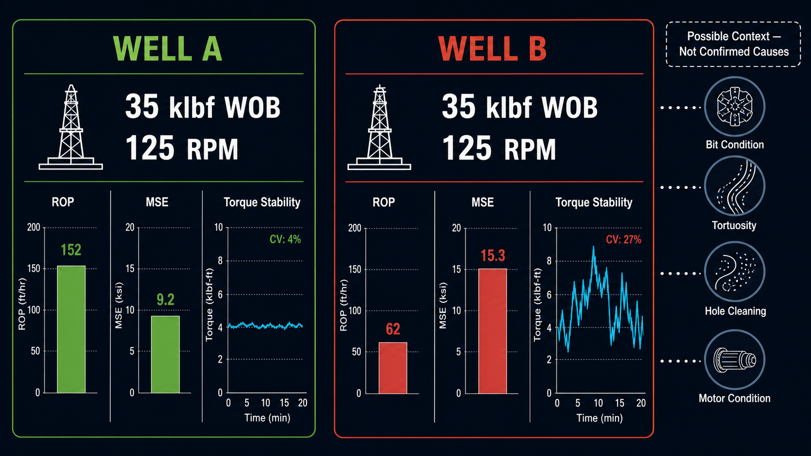
Similar WOB and RPM do not uniquely determine drilling response; bit, BHA, motor, and wellbore context still matter.

WOB and RPM Are Controls, Not Complete Descriptors

This distinction is fundamental.

The driller can directly control or influence:

• WOB,
• RPM,
• flow,
• differential pressure or ROP set point depending on the control mode.

Those are control variables.

Performance depends on those controls interacting with:

state variables that the driller cannot set directly.

Examples include:

• formation,
• bit wear,
• hole condition,
• trajectory,
• BHA behavior.

A WOB–RPM map therefore tells us:

What happened when these controls were used under the states represented by the dataset?

It does not tell us:

What must always happen whenever those controls are used.

Historical Heat Maps Can Suffer From Selection Bias

There is another statistical problem.

The historical dataset contains only the parameter combinations the crews actually chose.

Suppose the field historically operated conservatively around:

• 25–35 klbf,
• 100–130 RPM.

There may be no information about:

• 40 klbf,
• 150 RPM.

The heat map cannot determine whether that unexplored region is:

• excellent,
• dangerous,
• mechanically impossible.

No data is not bad performance.

It is simply unknown.

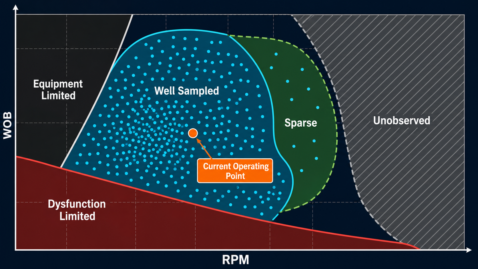
Unobserved parameter space is unknown, not necessarily poor, and must remain distinct from equipment and dysfunction limits.

This Creates an Exploration Problem

Optimization always contains some balance between:

exploitation

and:

exploration.

Exploitation

Operate where historical evidence already shows good performance.

Exploration

Try nearby parameter combinations to see whether performance can improve.

Too little exploration creates stagnation.

The rig repeatedly uses yesterday's parameters and may never discover better performance.

Too much exploration creates unnecessary operational variability and potential dysfunction.

In drilling, exploration must therefore be conservative and constrained.

A practical strategy is often:

1. start inside a historically strong region,
2. make controlled parameter changes,
3. observe the response,
4. move again only if the evidence supports it.

This is closer to local adaptive optimization than solving one global mathematical function.

Parameter Changes Should Be Treated as Experiments

Every intentional parameter change creates useful information.

Suppose the driller moves from:

32 klbf / 110 RPM

to:

35 klbf / 120 RPM.

The useful question is not simply:

Did ROP increase?

A richer observation includes:

• ROP response,
• MSE response,
• torque behavior,
• stick-slip evidence,
• differential pressure,
• persistence of the response.

The change becomes a small field experiment.

If the response improves:

the local landscape has been learned a little better.

If it deteriorates:

the previous region may be preferred.

This is one reason synchronized real-time data is so valuable.

Do Not Change WOB and RPM Simultaneously Unless You Accept Ambiguity

Suppose:

• WOB increases,
• RPM increases,
• ROP improves.

Which change caused the improvement?

We cannot know cleanly.

Operational reality sometimes requires multiple changes at once.

But from an analytical perspective, changing one parameter at a time provides much clearer information.

For example:

1. hold RPM approximately constant,
2. test a modest WOB change,
3. evaluate response,
4. then test RPM.

That resembles a field drill-off test more closely than randomly moving around the WOB–RPM plane.

The well determines how much experimentation is practical.

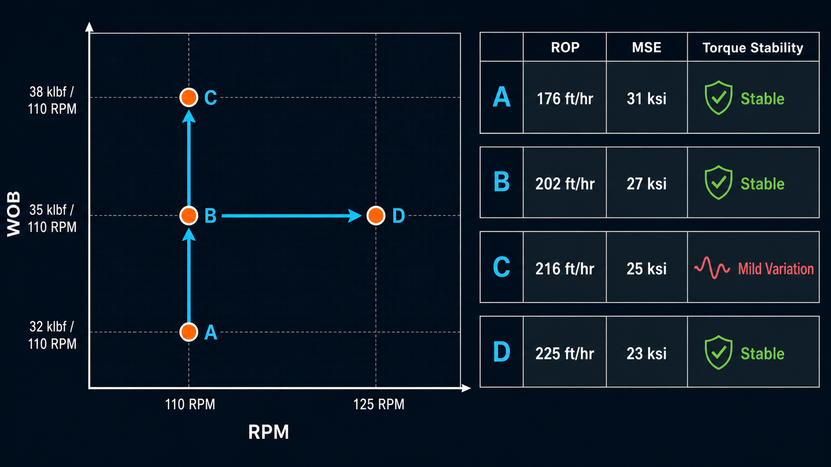
Controlled local changes reveal the current well’s response while preserving enough structure to interpret what changed.

Parameter Response Needs Time to Stabilize

Another subtlety is response lag.

Immediately after changing WOB:

• block control may settle,
• DOC changes,
• torque responds,
• ROP estimation may lag.

If the observation window is too short, the new operating point may be evaluated before the drilling system reaches a representative condition.

If the window is too long:

• formation may change,
• bit condition may change.

This connects back to the article on moving windows and meaningful change detection.

A parameter trial should be evaluated over a window long enough to represent stable drilling but short enough to preserve local context.

Operating Maps Need Boundaries

A performance surface should never exist without constraints.

Consider a region with excellent predicted ROP at:

• very high WOB,
• very high RPM.

Can the rig operate there?

Perhaps not.

Constraints may include:

• bit limits,
• motor differential pressure,
• motor RPM,
• top-drive torque,
• surface RPM,
• maximum SPP,
• vibration limits,
• directional requirements.

Therefore the useful map is not:

$$WOB \times RPM$$

alone.

It is:

$$Feasible\ WOB\text{-}RPM\ Region$$

within engineering constraints.

The Best Region Is Often a Plateau, Not a Point

Suppose performance is nearly identical across:

• WOB = 33–38 klbf,
• RPM = 120–140.

Why attempt to operate at exactly:

36.7 klbf / 132 RPM?

The apparent numerical precision is not useful.

A broad plateau can actually be operationally preferable because it provides:

• robustness to noise,
• flexibility for the driller,
• tolerance to natural variation.

The practical objective may be:

stay in the strong region

rather than:

hold the theoretical optimum point.

This is why parameter envelopes can be more useful than exact set points.

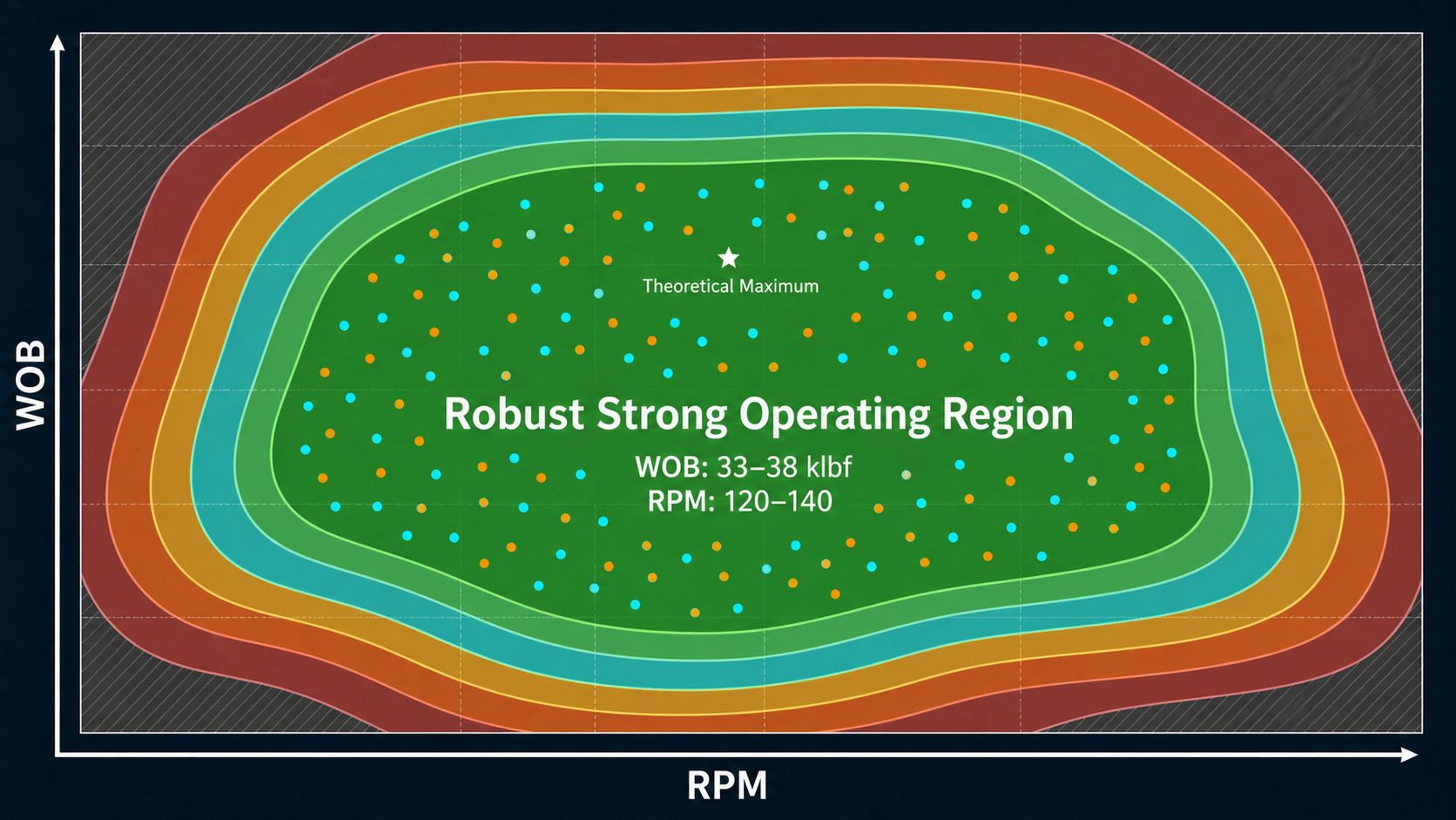
A broad stable plateau can be more useful operationally than one mathematically precise maximum.

A Local Optimum Can Be Good Enough

Optimization language sometimes makes "local optimum" sound like failure.

In drilling, a local optimum may be exactly what we want.

Suppose the rig has identified a region that provides:

• strong ROP,
• low MSE,
• stable torque,
• acceptable vibration.

There might be a slightly better theoretical region somewhere else.

Testing the path to it may introduce:

• dysfunction,
• unnecessary parameter cycling,
• equipment risk.

The marginal benefit may not justify the exploration.

Operational optimization should therefore consider the value of additional information versus the risk and cost of obtaining it.

Real-Time Evidence Should Override Historical Certainty

This is one of the strongest conclusions of SPE-186166.

Historical parameters can provide useful starting points.

But the paper cautions against assuming those points remain optimal and states that real-time data better reflects the actual conditions currently being drilled.[1]

That suggests a simple hierarchy:

Before entering the interval

Historical WOB–RPM data establishes the initial region.

Once drilling begins

The current well begins generating stronger local evidence.

As conditions evolve

The operating envelope should evolve too.

This mirrors the offset-benchmarking article:

history initializes the decision; the current well updates it.

A Practical Example

Consider a hypothetical lateral.

Historical offsets suggest a strong operating region around:

• WOB = 32–38 klbf,
• RPM = 115–135.

The current well starts at:

34 klbf / 120 RPM

and delivers:

• ROP = 205 ft/hr,
• stable torque,
• acceptable MSE.

The driller tests:

37 klbf / 120 RPM.

ROP increases to:

228 ft/hr.

MSE improves.

Torque remains stable.

Good evidence.

Next:

40 klbf / 120 RPM.

ROP reaches:

232 ft/hr,

but torque begins oscillating.

The additional 3 klbf generated only:

4 ft/hr

of additional ROP while worsening the mechanical response.

Now reduce WOB to:

37 klbf

and increase RPM to:

130.

ROP:

235 ft/hr

Torque stabilizes.

This locally appears stronger.

The lesson is not:

37 klbf / 130 RPM is optimal.

The lesson is:

Under the current formation, bit, BHA, and hole condition, the system responded favorably in the neighborhood of this operating point.

Five hundred feet later, the experiment may need to be repeated.

Heat Maps Should Be Treated as Evidence Maps

This may be the best way to interpret them.

A WOB–RPM map does not show:

the laws of the well.

It shows:

the performance observed—or estimated—from the available evidence.

A mature map should ideally convey:

• performance,
• dysfunction,
• data density,
• constraints,
• formation/context,
• current point.

The less context visible, the easier it is to overinterpret the colors.

A Real Parameter-Change Interval

When a WOB–RPM map is not available, depth-aligned traces can show the same nonlinear lesson without implying a product feature that does not exist. In this primary-well interval, the orange traces show ROP trending lower and MSE trending higher toward the end of the run. Stick-slip belief remains above 0.8 over the same interval, while MSE and the calculated rotary drilling-efficiency indicator show an inefficient mechanical response.

The BHA #3 label marks the trip. The bit was changed after wiped shoulder cutters were observed. These signals are consistent with deteriorating drilling response before the trip, but they should not be read as proof that one mechanism alone caused every change.

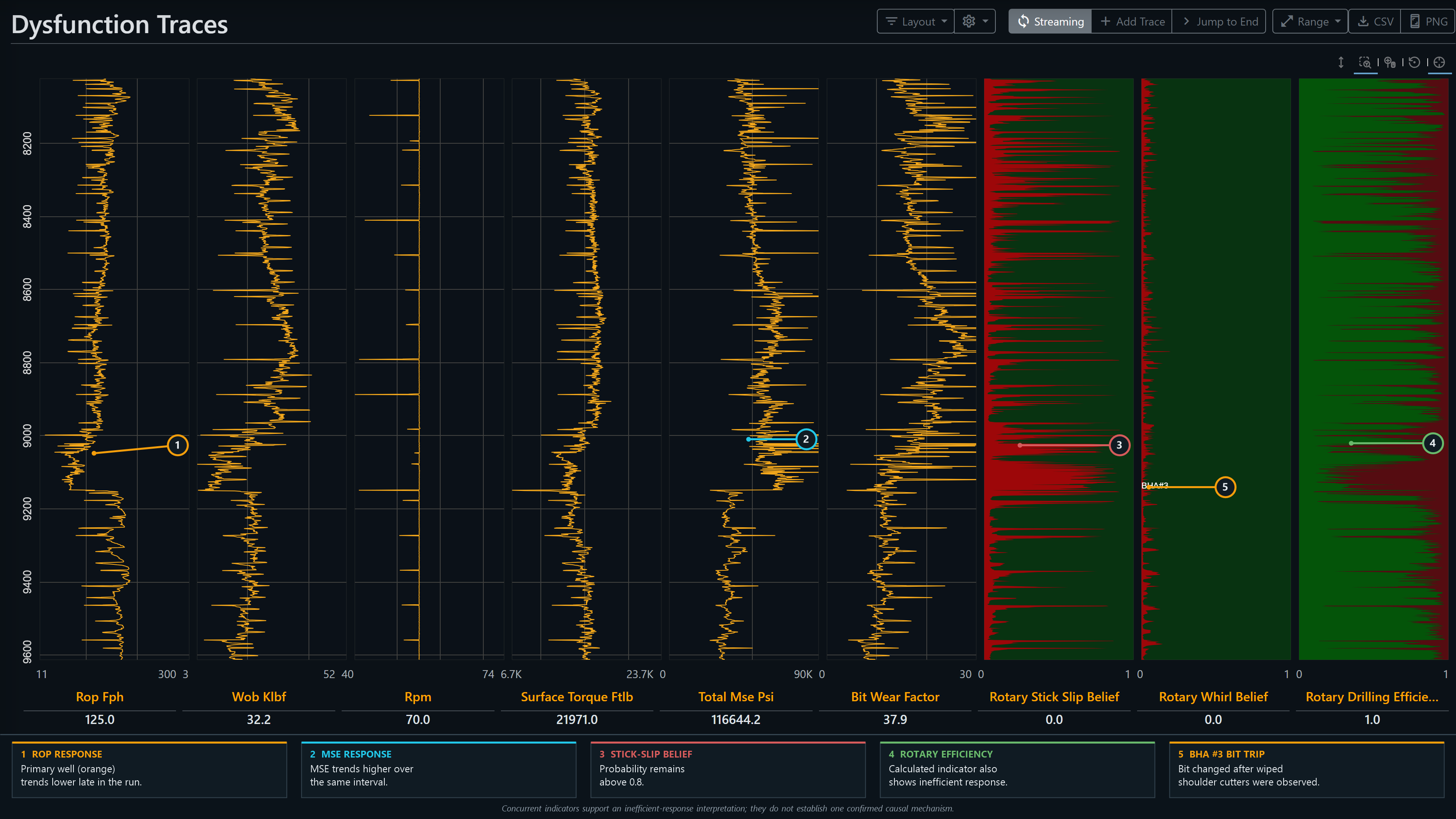
DrillingMetrics depth-aligned traces for the primary well. Before the BHA #3 trip, ROP trends lower while MSE rises, stick-slip belief stays above 0.8, and the calculated rotary drilling-efficiency indicator shows inefficient response. The trip replaced a bit with wiped shoulder cutters; the concurrent indicators support an inefficient-response interpretation but do not prove one isolated cause.

A Practical WOB–RPM Optimization Workflow

A defensible workflow might be:

1. Define the objective

Are we optimizing:

• ROP,
• MSE,
• drilling efficiency,
• mechanical stability?

2. Define the population

Filter by:

• rig state,
• formation,
• hole section,
• relevant BHA/bit context.

3. Plot observed operating points

Keep the raw evidence visible.

4. Attach performance and dysfunction

For each region, evaluate:

• ROP,
• MSE,
• torque behavior,
• dysfunction indicators.

5. Show data density

Avoid treating sparse interpolation as strong evidence.

6. Apply operational limits

Remove parameter regions that are not physically or operationally feasible.

7. Select a strong operating region

Prefer a robust plateau over a numerically precise point.

8. Make controlled local changes

Use the current well to learn the local response.

9. Reevaluate after context changes

Formation, bit condition, BHA behavior, and hole condition can move the landscape.

The Map Is a Snapshot of a Dynamic System

A WOB–RPM map is seductive because it makes drilling look like a static optimization problem.

It is not.

The operating landscape reflects:

$$Controls + Formation + Bit + BHA + Wellbore + Time$$

As those conditions evolve, the landscape evolves.

This is why field data can produce several high-performance clusters instead of one smooth optimum.

It is also why two nearby wells can respond differently to nearly identical parameter settings.

The parameter pair does not define the entire drilling system.

It defines where the driller is operating inside that system.

Conclusion

WOB and RPM are powerful drilling controls.

They are not independent knobs connected to a simple smooth ROP surface.

Their effect depends on:

• one another,
• formation,
• bit condition,
• BHA,
• hole cleaning,
• tortuosity,
• dysfunction,
• mechanical constraints.

That creates a performance landscape that can be:

• nonlinear,
• non-convex,
• sparse,
• time-varying.

The practical objective is therefore not necessarily to discover one global optimum.

A much more useful goal is to identify:

a strong, stable, mechanically acceptable operating region supported by current evidence—and continue updating that region as the well changes.

Historical maps tell us where previous wells succeeded.

Real-time data tells us whether those lessons still apply.

And controlled parameter changes allow the current well to teach us what its own performance landscape looks like.

That is a more realistic view of drilling optimization than searching for one perfect WOB and RPM pair.

---

References

1. Ambrus, A., Ashok, P., Chintapalli, A., Ramos, D., Behounek, M., Thetford, T. S., and Nelson, B. A Novel Probabilistic Rig Based Drilling Optimization Index to Improve Drilling Performance. SPE-186166-MS, SPE Offshore Europe Conference & Exhibition, Aberdeen, United Kingdom, 2017.

2. Behounek, M., Millican, B., Nelson, B., Wicks, M., Rintala, E., White, M., Thetford, T., Ashok, P., and Ramos, D. Change Management Challenges Deploying a Rig-Based Drilling Advisory System. SPE/IADC-194184-MS, SPE/IADC International Drilling Conference and Exhibition, The Hague, Netherlands, 2019.

3. Shahri, M., James, M., Vasicek, A., De Napoli, R., White, M., Behounek, M., D'Angelo, J., Ashok, P., and van Oort, E. Case Studies: Optimizing BHA Performance by Leveraging Data and Advanced Modeling. SPE-196020-MS, SPE Annual Technical Conference and Exhibition, Calgary, Alberta, 2019.