Mechanical Specific Energy: Powerful Metric, Incomplete Diagnosis

MSE compresses WOB, torque, RPM, and ROP into a physically meaningful measure of drilling energy. Its strength is detecting inefficiency; its limitation is that many different drilling conditions can produce the same response.

Suppose MSE increases sharply while drilling.

What happened?

Possibilities include:

• the formation became harder,
• ROP deteriorated,
• torque increased,
• stick-slip developed,
• the bit began drilling inefficiently,
• hole cleaning deteriorated,
• bit hydraulics became less effective,
• the bit started wearing,
• operating parameters changed.

All of those can alter MSE.

That is simultaneously the metric's greatest strength and its greatest limitation.

Mechanical Specific Energy combines several important drilling measurements into one quantity representing the mechanical energy required to remove a unit volume of rock.

That makes MSE unusually useful for answering:

Is the drilling system using mechanical energy efficiently?

It is much less capable, by itself, of answering:

Why is the system inefficient?

That distinction matters.

SPE-186166 notes that MSE trends are useful for identifying inefficient drilling and drilling dysfunctions, while also emphasizing that the type of dysfunction may not be evident from the MSE trend alone.[1]

The paper gives an especially important reason: different dysfunctions may require very different—and sometimes opposing—parameter changes.

A metric that tells us:

efficiency deteriorated

is therefore not automatically a metric that tells us:

reduce WOB

or:

increase RPM.

The engineering value of MSE increases significantly when it is treated as evidence of changing drilling behavior rather than a complete diagnostic system.

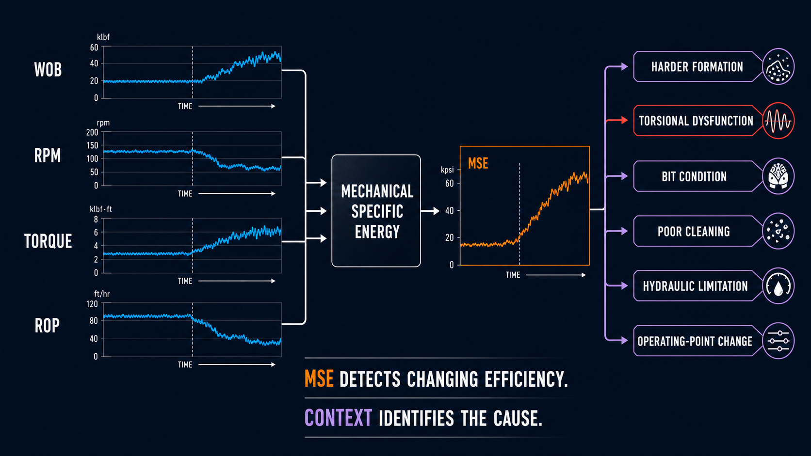
MSE is a strong efficiency signal, but the same rise can have several physical explanations.

What MSE Actually Measures

At its core, specific energy asks:

How much mechanical work is being applied for each unit volume of rock removed?

Because energy divided by volume has the same dimensions as pressure, MSE is often expressed in units such as psi.

A commonly used surface formulation can be written as:

$$MSE = \frac{WOB}{A_b} + \frac{120\pi N T} {A_b \cdot ROP}$$

where:

• (WOB) = weight on bit,
• (A_b) = bit area,
• (N) = rotary speed,
• (T) = torque,
• (ROP) = rate of penetration.

The exact form and unit conversions depend on the implementation, but the physical structure is the important part.

There are two major mechanical contributions.

Axial contribution

$$\frac{WOB}{A_b}$$

This represents the axial loading applied over the bit area.

Rotational contribution

$$\frac{120\pi N T} {A_b \cdot ROP}$$

This represents rotational work relative to the volume of hole being created.

MSE therefore combines:

how hard the bit is being loaded

with:

how much rotational work is being applied

and asks:

how much rock is being removed in return?

That makes it fundamentally different from ROP alone.

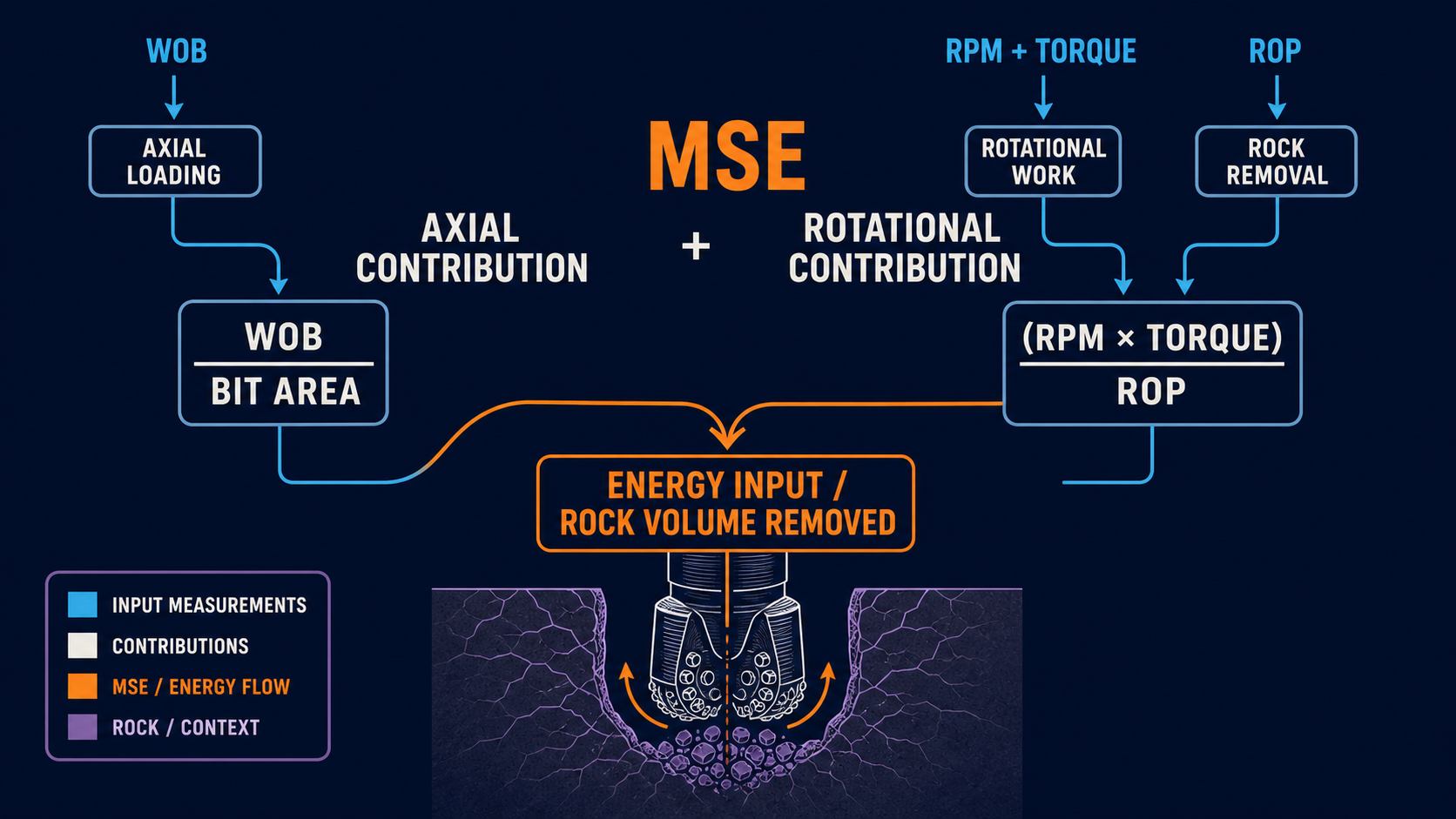
MSE combines axial loading and rotational work relative to the volume of rock removed.

ROP Measures Speed; MSE Measures Energy Efficiency

Consider two drilling intervals.

Interval A

ROP:

250 ft/hr

with very high:

• WOB,
• RPM,
• torque.

Interval B

ROP:

220 ft/hr

with materially less mechanical input.

Which interval represents better drilling performance?

ROP alone favors Interval A.

MSE may reveal that Interval B is removing nearly as much rock while requiring considerably less mechanical work per unit volume.

That does not automatically make Interval B the preferred operating condition.

But it exposes something ROP does not:

the energetic cost of achieving the penetration rate.

This is why MSE became so useful for drilling optimization.

It converts several surface parameters into one physically interpretable performance quantity.

MSE Is Extremely Sensitive to ROP

One of the most important features of the equation is easy to overlook.

ROP is in the denominator of the rotational term:

$$MSE_{rot} \propto \frac{N T}{ROP}$$

Suppose:

• RPM stays constant,
• torque stays constant,
• WOB stays constant.

Now ROP falls by half.

The rotational contribution to MSE approximately doubles.

No additional rotational energy is being applied.

The drilling system is simply removing less rock with the same energy input.

That is exactly the inefficiency MSE is intended to expose.

But it also creates an interpretive issue.

A formation change that legitimately reduces ROP can cause a large MSE increase even if nothing mechanically unhealthy has happened.

SPE-205844 makes a related point while discussing a different mechanics-based metric: quantities that depend strongly on ROP can change because of formation or dysfunction even when the equipment condition being investigated has not changed.[2]

That same caution is essential when interpreting MSE.

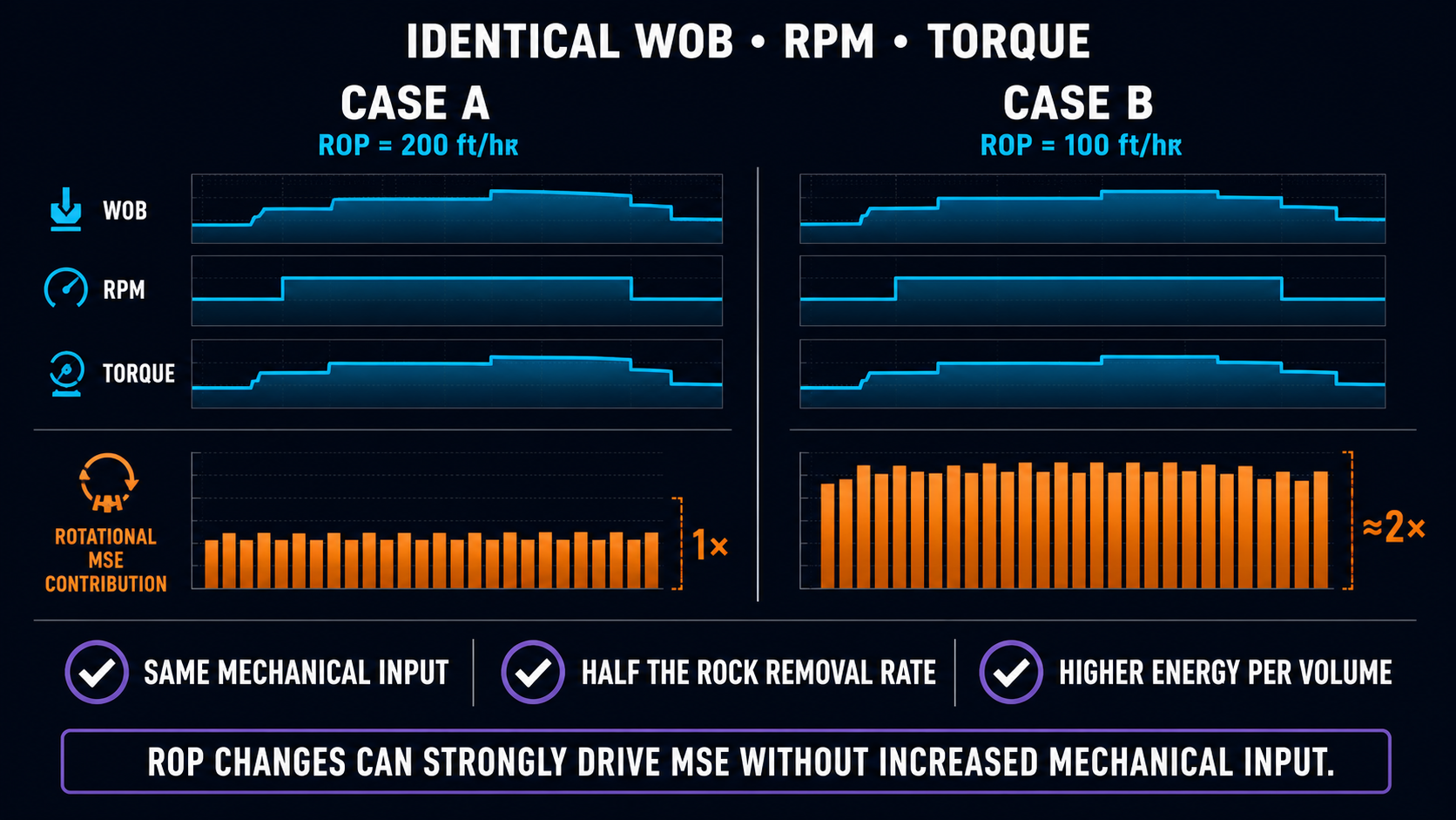
With the same mechanical input, halving ROP approximately doubles the rotational MSE contribution.

A High MSE Value Is Not Automatically a Dysfunction

Suppose MSE rises while entering a harder formation.

The bit now requires more work to remove the same volume of rock.

MSE should rise.

That may be completely normal.

Now suppose MSE rises in a homogeneous formation while:

• WOB remains stable,
• RPM remains stable,
• torque becomes severely oscillatory,
• ROP falls.

That is a different situation.

Both cases may produce:

high MSE.

Only the second contains obvious additional evidence of drilling dysfunction.

This is why absolute MSE should usually be interpreted relative to:

• formation,
• recent baseline,
• historical offsets,
• operating state,
• drilling parameters.

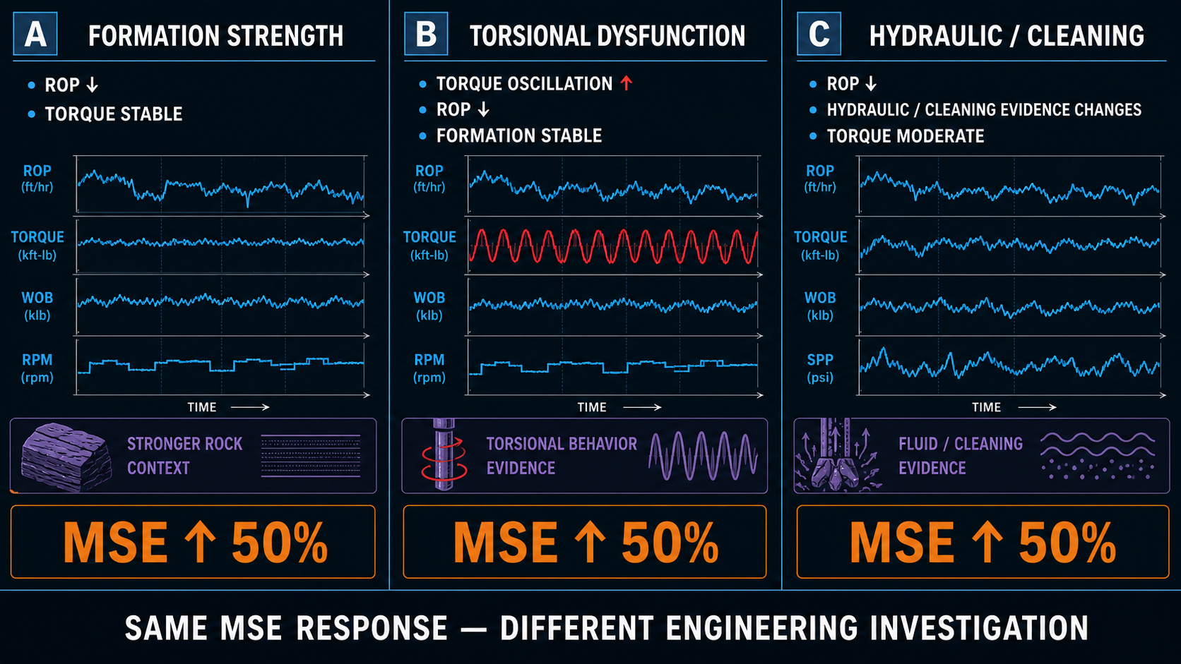
The same MSE increase can lead to different investigations when the supporting evidence changes.

Formation Strength Provides Critical Context

The conceptual relationship between rock strength and specific energy is powerful.

If two intervals require very different energy per unit volume, one possible explanation is simply that the rock is different.

SPE-186166 therefore combines MSE with formation-strength information when available rather than interpreting MSE independently.[1]

The useful comparison is not always:

$$MSE_{current} \quad vs. \quad MSE_{previous}$$

It may instead be closer to:

$$MSE \quad relative\ to\ expected\ rock\ strength$$

If MSE rises at approximately the same time that the formation becomes substantially stronger, the change may be expected.

If MSE rises sharply while the rock-strength context remains similar, the evidence for mechanical inefficiency becomes stronger.

The difficulty is that formation strength is itself often uncertain.

Possible inputs might include:

• UCS estimates,
• CCS estimates,
• log-derived rock properties,
• formation classification,
• offset behavior.

So even formation-normalized MSE should not be treated as exact truth.

It improves context.

It does not eliminate uncertainty.

One Universal MSE Threshold Is Usually Too Simple

It is tempting to establish:

MSE above X psi = inefficient.

That can be useful within a tightly controlled operating context.

Across a whole well or field, it becomes much harder to defend.

Normal MSE can change because of:

• formation strength,
• hole size,
• bit type,
• BHA,
• drilling mode,
• bit condition,
• downhole motor contribution.

A better surveillance architecture often uses a contextual baseline.

For example:

What MSE range has been normal for rotary drilling with this BHA in this formation?

That question is considerably more useful than:

Is MSE above a global threshold?

MSE Is Also Not a Dysfunction Classifier

This distinction is especially important.

Suppose MSE is elevated.

Possible dysfunctions include:

• stick-slip,
• whirl,
• bit bounce,
• bit balling.

The MSE response can overlap substantially among these conditions.

SPE-186166 explicitly warns that the dysfunction type may not be evident from MSE trend analysis alone.[1]

Why does that matter?

Because dysfunction mitigation is not generic.

The same paper points out that parameter changes appropriate for stick-slip may differ from those appropriate for whirl.

The exact response must still consider:

• BHA,
• bit,
• formation,
• control system,
• operating limits.

The key lesson is simpler:

High MSE does not contain enough diagnostic information to determine the corrective parameter move by itself.

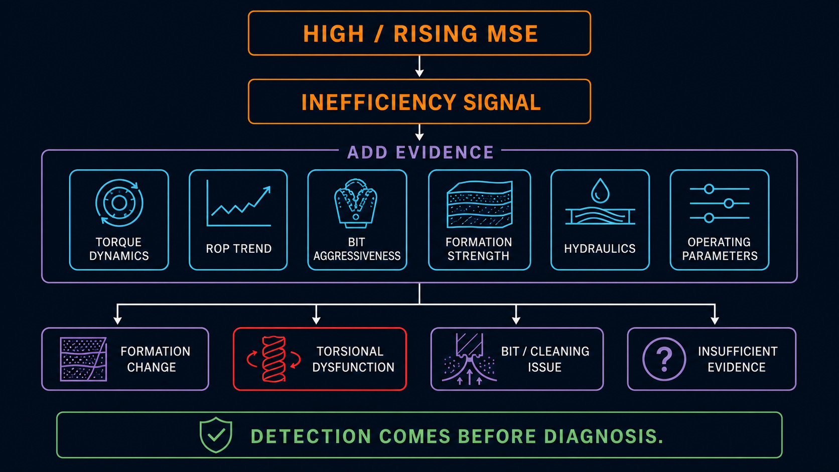
MSE detects changing efficiency; diagnosis requires independent evidence.

Torque Behavior Adds Diagnostic Information

Consider two high-MSE intervals.

Interval A

Torque is high but stable.

Interval B

Torque oscillates dramatically.

The MSE magnitude may be similar.

The underlying mechanical behavior is clearly not.

Torque dynamics provide information that the scalar MSE value has compressed away.

This reveals a general limitation of composite metrics.

Whenever several inputs are collapsed into one output, some of the structure of the original signals is lost.

MSE is useful partly because it simplifies several channels.

But when the result becomes abnormal, the engineer often needs to return to the original channels.

That makes a good workflow:

$$Raw\ Signals \rightarrow MSE \rightarrow Detect\ Change \rightarrow Return\ to\ Raw\ Evidence$$

rather than:

$$MSE \rightarrow Automatic\ Diagnosis$$

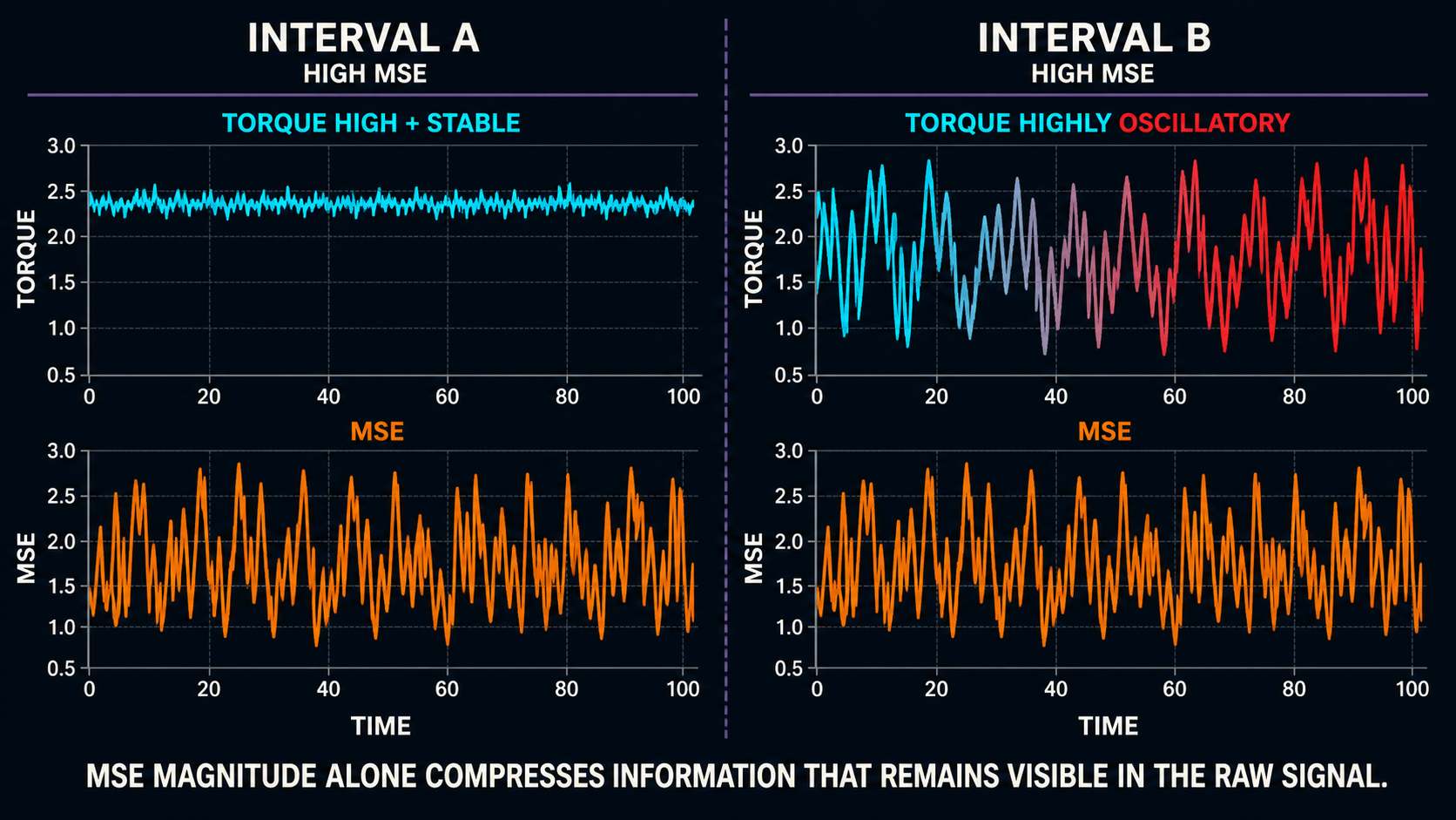
Similar MSE magnitude can conceal materially different torque dynamics.

Bit Aggressiveness Can Help Separate Behaviors

Another mechanics-based quantity is bit aggressiveness.

Conceptually, it relates torque to WOB and bit size.

While MSE tells us about mechanical energy per volume removed, aggressiveness helps characterize the relationship between:

• axial loading,
• rotational resistance.

A rising MSE accompanied by falling bit aggressiveness can represent a different mechanical state from:

rising MSE accompanied by rising aggressiveness.

This is one reason SPE-186166 combines multiple derived quantities rather than using MSE as the only input to drilling-efficiency analysis.[1]

The broader lesson is important:

Multiple partially independent mechanical indicators can preserve information that one composite KPI cannot.

MSE and Torque Oscillation Should Not Be Counted as Fully Independent

There is another statistical subtlety.

MSE already contains torque.

If an analytical system uses:

• MSE,
• torque,
• a torque-derived stick-slip indicator,

those are not three fully independent measurements.

They share information.

This does not make the combination invalid.

It means the analyst should understand the dependency structure.

Likewise, ROP is embedded directly in MSE.

If ROP falls and MSE rises, those are partially mathematically coupled observations.

A statement such as:

ROP fell and MSE rose

is useful.

But it is not the same as observing two completely independent symptoms.

Hydraulics Can Affect MSE Without Appearing Explicitly in Surface MSE

The classic surface MSE equation is mechanical.

It does not directly include the hydraulic energy delivered at the bit.

But hydraulics can strongly affect drilling efficiency.

Poor bit cleaning can reduce ROP.

That lower ROP then raises MSE.

From the MSE trace alone, the problem may appear mechanical even though ineffective cleaning is contributing to the deterioration.

This motivated extensions such as:

• Hydro-Mechanical Specific Energy,
• Drilling Specific Energy,

which attempt to account for hydraulic energy as well.

SPE-186166 notes that adding hydraulic context can improve identification of dysfunction associated with poor hydraulics management.[1]

This does not mean every MSE workflow should simply add hydraulic horsepower to the equation.

It means:

if hydraulics can influence the phenomenon being diagnosed, hydraulics should be part of the interpretation.

Hole Cleaning Can Alter the Mechanical Response Indirectly

Poor hole cleaning provides another example.

Cuttings accumulation can affect:

• weight transfer,
• torque,
• drag,
• ROP.

All of those can influence the apparent drilling efficiency.

A high MSE response may therefore be a symptom of a larger wellbore condition problem rather than a purely bit-rock interaction problem.

This is one reason long-horizon hole-cleaning surveillance requires operational history rather than relying only on instantaneous drilling efficiency.

MSE sees the current energetic result.

It does not know the previous several hours of:

• circulation,
• static time,
• reaming,
• pipe rotation.

That historical context lives elsewhere.

MSE Can Change Because the Bit Is Changing

Bit condition is another important confounder.

A sharp or progressive deterioration in bit cutting effectiveness can reduce ROP even if surface parameters remain similar.

MSE rises.

That makes MSE potentially useful for recognizing deterioration.

But again:

MSE increase does not prove bit wear.

SPE-205844 explicitly notes that formation and dysfunction can alter ROP-dependent mechanics metrics even in the absence of PDC wear or damage.[2]

The authors therefore combined mechanical metrics with:

• stand-level trends,
• surface-data review,
• post-run dull information

when investigating PDC damage.

The same discipline is useful for MSE.

Surface MSE and Downhole MSE Are Not the Same Thing

The earlier article on surface versus downhole measurements becomes particularly relevant here.

Standard surface MSE commonly uses:

• surface RPM,
• surface torque,
• surface WOB.

With a mud motor, especially while sliding:

$$RPM_{surface} \neq RPM_{bit}$$

Likewise:

surface torque is not necessarily torque at bit.

SPE-186166 describes separate treatment when a downhole motor is present, where estimated motor-generated RPM and torque can be incorporated rather than relying only on surface rotary quantities.[1]

This means a field labeled simply:

MSE

can be ambiguous.

Useful metadata might distinguish:

• surface MSE,
• motor-adjusted MSE,
• modeled downhole MSE.

Those values should not automatically be benchmarked together.

Rotary and Slide MSE Should Not Be Blindly Compared

Suppose:

Rotary drilling

Surface RPM = 120.

Slide drilling

Surface RPM = 0.

A classic surface rotational term will behave completely differently.

But the motor may still be rotating the bit rapidly during the slide.

Comparing the two MSE values without accounting for motor mechanics can create a misleading result.

This is another example of the broader analytical rule:

compare operating populations that represent the same physical process.

Rotary drilling and slide drilling should generally be treated separately unless the calculation methodology explicitly makes them comparable.

Smoothing Helps—Until It Hides the Event

Raw MSE can be noisy because several of its inputs are noisy.

Torque fluctuates.

ROP fluctuates.

WOB fluctuates.

The ratio can therefore become very erratic.

Moving averages or depth-based aggregation can make the trend much easier to interpret.

SPE-186166 uses both instantaneous and trend/movement information, with moving-window methods used to characterize whether derived drilling parameters are increasing, decreasing, constant, or erratic.[1]

But the earlier change-detection article highlighted the danger:

too much smoothing can suppress real short-duration mechanical events.

The correct window depends on the question.

Formation-scale efficiency

A depth-based moving average may be useful.

Stand-level bit deterioration

A stand median may be useful.

Short dysfunction event

High-frequency time data may be necessary.

There is no universally correct MSE smoothing interval.

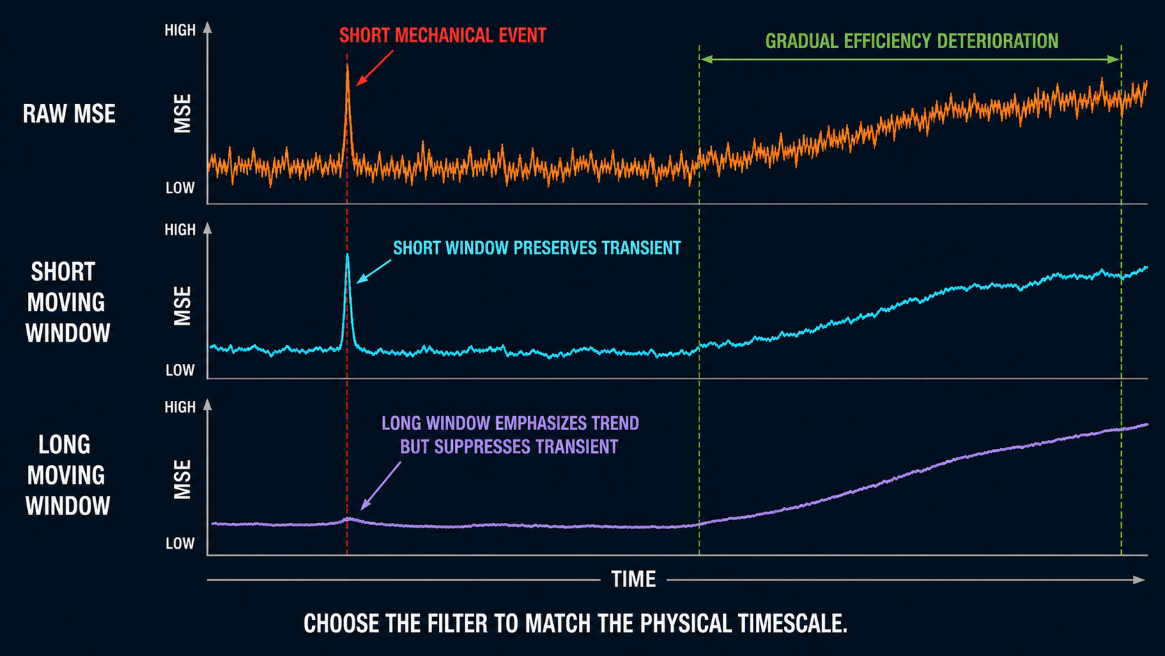
Short windows preserve transients, while long windows emphasize slower deterioration.

MSE Trend Is Often More Useful Than MSE Magnitude

Consider two formations.

Formation A normally drills around:

25 ksi MSE

Formation B normally drills around:

55 ksi MSE

If the current MSE is:

45 ksi

is that good?

The answer depends on location.

In Formation A, 45 may represent substantial deterioration.

In Formation B, it may represent efficient performance.

This suggests that the most useful quantity may sometimes be:

$$\Delta MSE = MSE_{current} - MSE_{expected}$$

where expected MSE is derived from:

• recent healthy operation,
• formation-specific history,
• offset wells,
• a modeled relationship.

The important concept is not the particular subtraction.

It is the move from:

absolute value

toward:

departure from a relevant baseline.

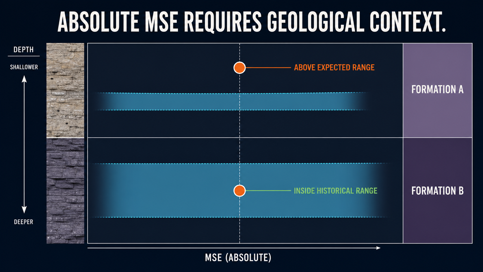
An identical MSE value can be abnormal in one formation and expected in another.

MSE Can Be Very Useful in Offset Benchmarking

Once the population has been normalized properly, MSE becomes a useful offset metric.

For example, compare:

• same formation,
• same hole size,
• rotary drilling only,
• similar BHA and bit,
• comparable depth.

Now the engineer can ask:

Which wells removed the rock with the least mechanical energy?

That adds information beyond ROP.

One offset may have drilled faster but with:

• much higher torque,
• substantially higher WOB,
• more dysfunction.

Another may have achieved similar footage with a cleaner energy response.

That is useful when selecting a starting operating envelope for the current well.

But the offset article's warning still applies:

historical MSE is evidence, not a universal target.

WOB-RPM Optimization Is Nonlinear

Another common temptation is to use MSE to construct a smooth optimization surface:

$$MSE=f(WOB,RPM)$$

and then select the minimum.

Real drilling is more complicated.

SPE-186166 found drilling-performance regions in WOB-RPM space to be highly nonlinear and non-convex.[1]

Even similar WOB/RPM combinations produced materially different drilling efficiency on nearby wells because of factors such as:

• bit condition,
• tortuosity,
• hole cleaning,
• motor condition.

Therefore:

the same parameter pair does not guarantee the same MSE response.

The operating landscape evolves as the system evolves.

Low MSE Does Not Capture Every Definition of a Good Well

Even if MSE is low, another performance objective may still be poor.

For example:

• wellbore tortuosity may be excessive,
• directional control may be poor,
• hole quality may be compromised,
• equipment may be operating near a limit.

SPE-196020 makes the broader point that traditional performance metrics such as ROP and total days do not fully represent wellbore quality, and that the highest-ROP well may not necessarily be the best completion or production well.

The same applies to MSE.

MSE measures something important.

It does not measure everything important.

A Practical Example: Three Identical MSE Increases

Consider three hypothetical stands.

In each case:

MSE rises approximately 50% relative to the previous baseline.

Case A — Formation Change

Observed:

• ROP falls,
• torque increases moderately,
• WOB and RPM remain stable,
• torque remains smooth.

Context:

• formation marker changes,
• offsets show similar ROP deterioration.

Interpretation:

The MSE increase is substantially consistent with increased rock strength.

Case B — Torsional Dysfunction

Observed:

• ROP falls,
• torque becomes highly oscillatory,
• WOB/RPM set points remain stable,
• no known formation transition occurs.

Interpretation:

MSE indicates deteriorating efficiency.

Torque dynamics provide additional evidence of a torsional problem.

Case C — Cleaning / Hydraulic Concern

Observed:

• ROP progressively deteriorates,
• MSE rises,
• torque behavior changes only modestly,
• hydraulic / circulation evidence also begins changing.

Interpretation:

MSE confirms poorer drilling efficiency.

The cause cannot be determined from MSE alone; hydraulic and hole-condition evidence deserves investigation.

All three cases have:

the same headline result:

MSE increased 50%.

The appropriate engineering response is different in each.

That is the central limitation of interpreting MSE without context.

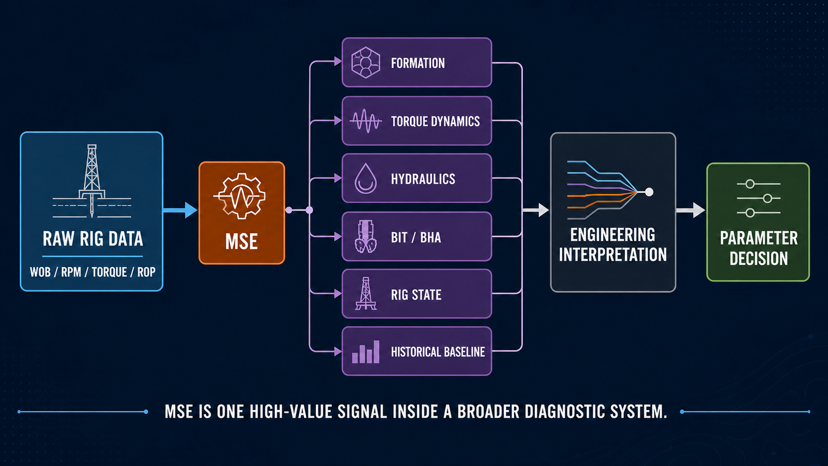
MSE becomes diagnostic only when combined with formation, dynamics, hydraulics, operating state, and historical context.

A Better Real-Time MSE Workflow

A practical workflow might look like this.

1. Confirm rig state

Only compare physically compatible drilling modes.

2. Calculate the appropriate MSE

Distinguish:

• surface,
• motor-adjusted,
• other methodology.

3. Establish a contextual baseline

Use:

• formation,
• recent depth,
• offset distribution,
• similar BHA/bit context.

4. Detect the departure

Evaluate:

• magnitude,
• rate of change,
• persistence,
• erratic behavior.

5. Return to the source channels

Review:

• WOB,
• RPM,
• torque,
• ROP.

6. Add independent evidence

Examples:

• torque oscillation,
• differential pressure,
• hydraulics,
• bit aggressiveness,
• formation strength,
• hole-cleaning history.

7. Separate detection from diagnosis

Ask:

Has drilling efficiency changed?

before asking:

Why?

8. Make the recommendation only after diagnosis

Do not derive a parameter change directly from MSE magnitude alone.

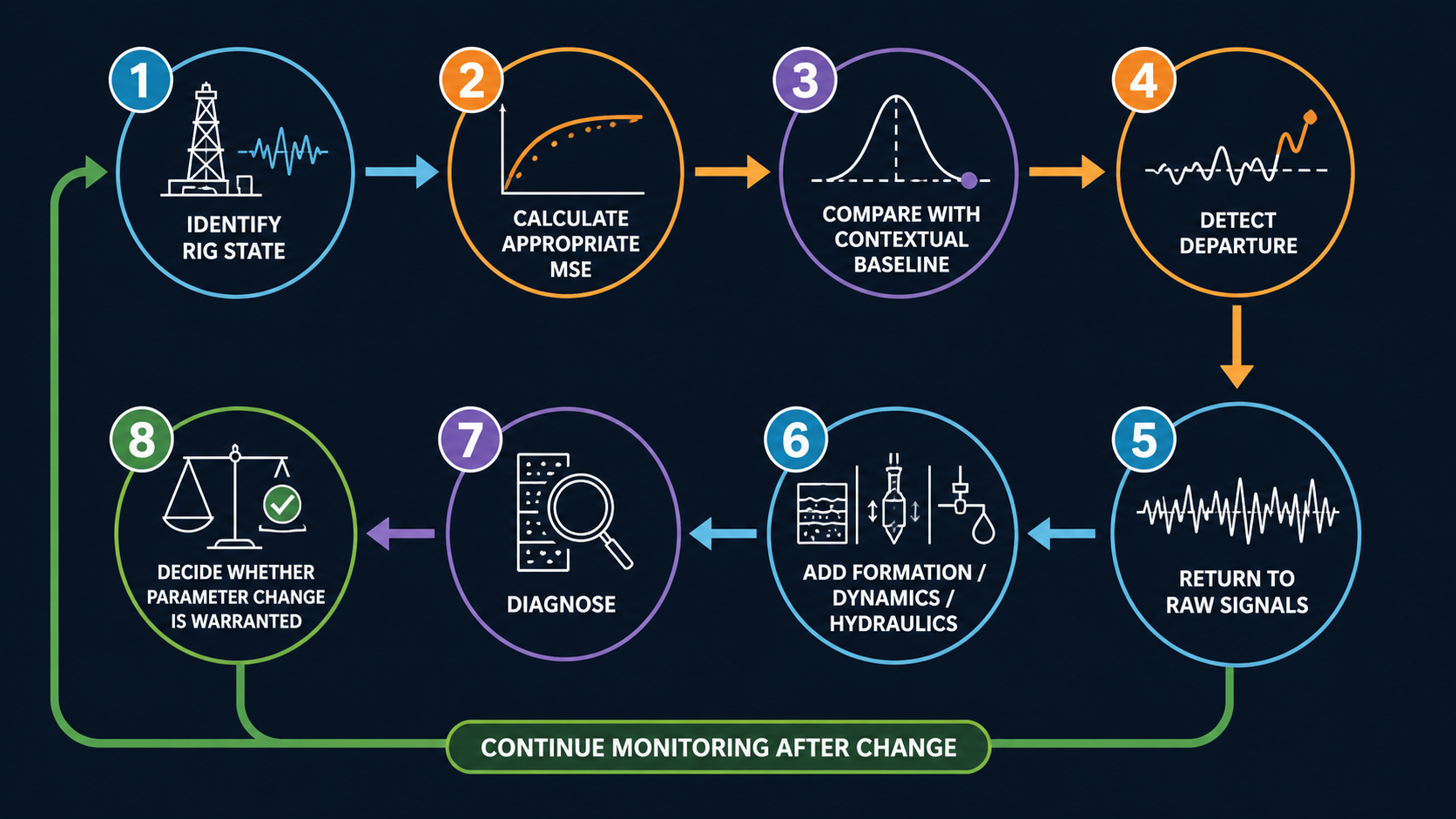
A practical MSE workflow detects a departure, returns to the raw signals, adds context, and then decides whether a parameter change is warranted.

MSE in a Real Depth-Based Comparison

The depth-based DrillingMetrics comparison below keeps the constituent signals beside MSE rather than treating it as an isolated KPI.

The orange trace is the primary well, the blue trace is a same-pad offset, and the green bands show parameter ranges from a selected group of comparable wells. BHA #3 marks a bit trip on the primary well.

Before the trip, the primary well trends toward higher MSE and lower ROP through the section. After the trip, ROP and MSE move back toward the selected-well trend. Depth of cut also begins to decline toward the end of the run.

The figure does not prove that the bit trip alone caused the change. It does show why MSE is more useful when ROP, operating parameters, an offset trace, and a historical range remain visible.

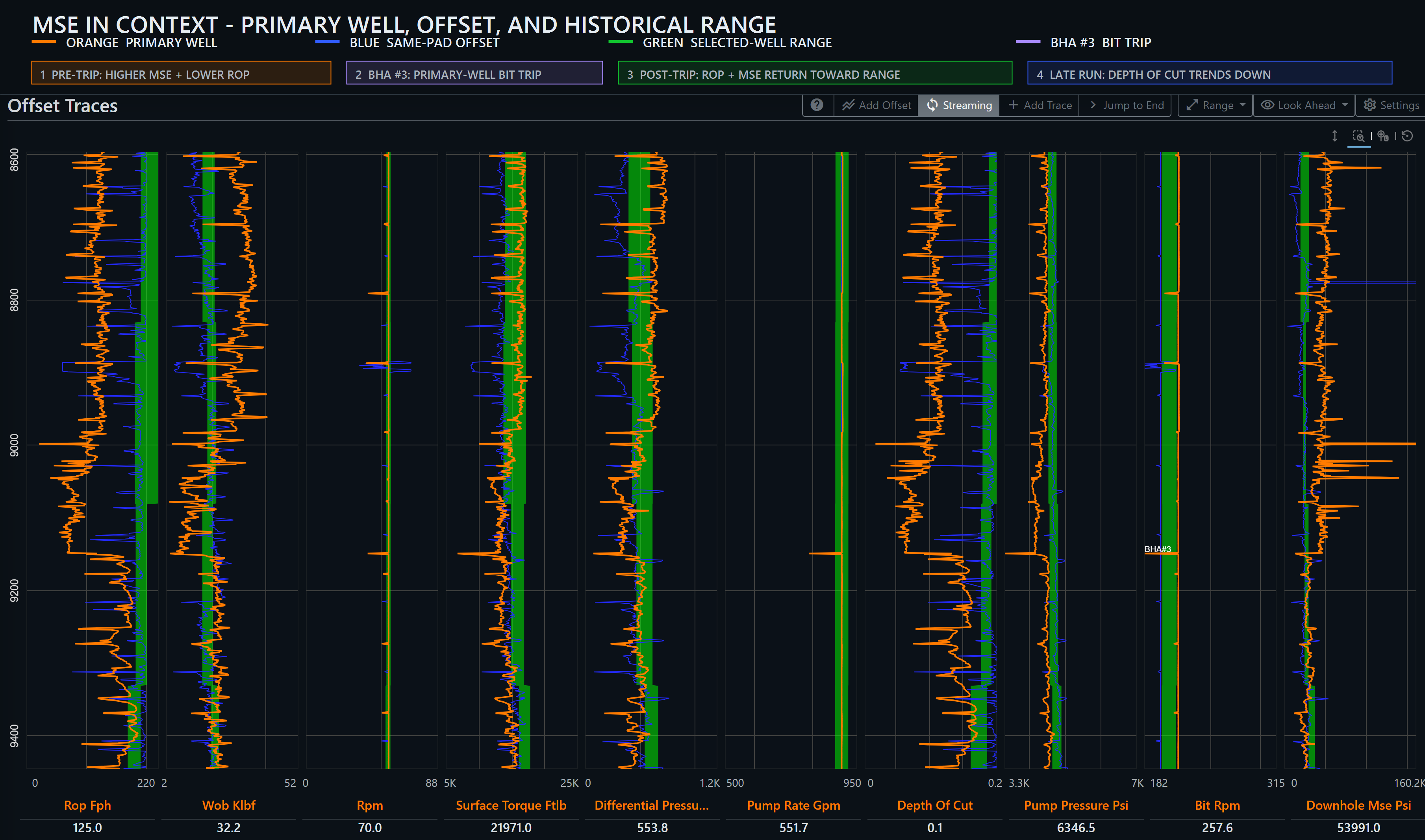
Depth-based comparison of the primary well (orange), same-pad offset (blue), and selected-well parameter ranges (green).

What MSE Is Best At

MSE is especially powerful for:

Identifying deteriorating energy efficiency

It can expose situations where mechanical input remains high while rock removal becomes less effective.

Comparing parameter combinations

It provides more context than ROP alone.

Detecting departures from a baseline

A changing MSE trend can direct the engineer toward an interval worth investigating.

Combining several drilling signals

It compresses WOB, RPM, torque, and ROP into one physically interpretable quantity.

Those are significant strengths.

What MSE Is Not

MSE is not automatically:

A rock-strength measurement

Formation strength influences MSE, but the two are not equivalent under inefficient drilling.

A dysfunction classifier

Several different dysfunctions can create similar MSE responses.

A bit-wear measurement

Bit deterioration may influence MSE, but formation and dysfunction can do the same.

A universal optimization target

The lowest instantaneous MSE does not necessarily produce the best total well outcome.

A substitute for the raw traces

Once MSE becomes unusual, the original channels often contain the information needed for diagnosis.

The Most Useful Question Is Not "Is MSE High?"

Instead ask:

Is MSE higher than we would expect under the current drilling conditions?

And if the answer is yes:

Which independent evidence explains the difference?

Those questions transform MSE from a dashboard number into an engineering surveillance tool.

Conclusion

Mechanical Specific Energy remains one of the most useful quantities available from ordinary drilling data.

Its appeal is easy to understand.

It takes:

• WOB,
• RPM,
• torque,
• ROP

and reduces them to a physical measure of mechanical energy per volume of rock removed.

That allows engineers to identify drilling conditions in which more mechanical work is producing less useful drilling progress.

But the compression has a cost.

The MSE value does not preserve all the information contained in the original measurements.

A rise in MSE may reflect:

• stronger rock,
• poor bit performance,
• torsional dysfunction,
• inadequate cleaning,
• changing hydraulics,
• equipment condition,
• or several effects simultaneously.

That is why the most effective use of MSE is not:

High MSE means X.

It is:

MSE has changed. What else changed with it?

Used that way, MSE becomes exactly what it should be:

a powerful real-time indicator of drilling efficiency that directs engineering attention toward the evidence needed for diagnosis.

---

References

1. Ambrus, A., Ashok, P., Chintapalli, A., Ramos, D., Behounek, M., Thetford, T. S., and Nelson, B. A Novel Probabilistic Rig Based Drilling Optimization Index to Improve Drilling Performance. SPE-186166-MS, SPE Offshore Europe Conference & Exhibition, Aberdeen, United Kingdom, 2017.

2. Witt-Doerring, Y., Pastusek, P. P., Ashok, P., and van Oort, E. Quantifying PDC Bit Wear in Real-Time and Establishing an Effective Bit Pull Criterion Using Surface Sensors. SPE-205844-MS, SPE Annual Technical Conference and Exhibition, 2021.

3. Dupriest, F. E., and Koederitz, W. L. Maximizing Drill Rates with Real-Time Surveillance of Mechanical Specific Energy. SPE-92194-MS, SPE/IADC Drilling Conference, Amsterdam, 2005.

4. Teale, R. The Concept of Specific Energy in Rock Drilling. International Journal of Rock Mechanics and Mining Sciences & Geomechanics Abstracts, Vol. 2, No. 1, 1965.