Real-Time Torque and Drag Is a Calibration Problem, Not Just a Modeling Problem

The equations behind torque and drag are well established. The harder real-time problem is continuously reconciling the model with actual hook load, torque, drillstring properties, friction, trajectory, and operational state.

Torque-and-drag modeling is not new.

For decades, drilling engineers have used mechanical models to estimate:

• pick-up weight,
• slack-off weight,
• rotating off-bottom torque,
• drag while tripping,
• friction factors,
• and the mechanical limits of extended-reach wells.

Running those calculations before a well is drilled is useful.

Running them after a problematic trip can also be useful.

But a real-time torque-and-drag model has a more demanding job.

It has to answer:

Does the mechanical behavior we are measuring right now agree with what this well should be doing?

That requires more than running the equations repeatedly.

The model has to know:

• the current well trajectory,
• what is in the drillstring,
• where the casing ends,
• the mud weight,
• how much the actual pipe weighs,
• the block-weight offset,
• whether the rig is picking up, slacking off, rotating, or doing something else,
• and what friction is consistent with the measurements already observed.

If those inputs are wrong, the model may calculate perfectly and still give the wrong answer.

This is why real-time torque and drag is fundamentally a calibration problem as much as a modeling problem.

SPE-191426 describes a field implementation in which a 3D soft-string model was integrated with real-time rig measurements and contextual data, then automatically calibrated so that measured hook load and torque could be interpreted against a continuously updated mechanical baseline.[1]

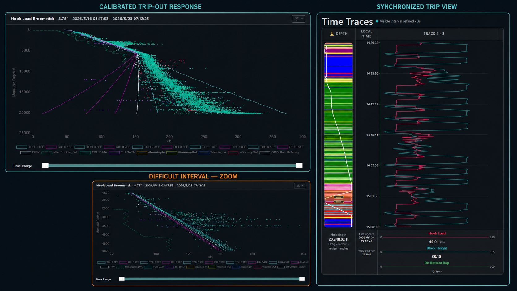
Real-time torque-and-drag analysis requires continuously reconciling a physics model with the actual drillstring, wellbore, and measured mechanical response.

What a Torque-and-Drag Model Actually Predicts

At its core, torque-and-drag modeling describes how forces are transmitted through a drillstring in a wellbore.

The drillstring has:

• buoyant weight,
• axial tension or compression,
• contact forces against the hole,
• friction at those contacts,
• and, when rotating, torque required to overcome mechanical resistance.

A common soft-string representation treats sliding friction conceptually as:

$$ F_f = \mu N $$

where:

• (F_f) is friction force,
• (\mu) is the friction factor,
• (N) is normal contact force.

The normal force itself depends on:

• trajectory,
• drillstring weight,
• tension,
• inclination,
• curvature,
• and other mechanical conditions.

Integrating those forces along the drillstring produces estimates of what should be measured at surface.

For example:

Pick-up

When pulling the string upward, friction resists upward movement.

Surface hook load should therefore be higher than the static string weight.

Slack-off

When lowering the string, friction acts in the opposite direction.

Surface hook load should therefore be lower.

Rotating off bottom

Rotation changes the frictional response and creates another observable condition that can be compared with modeled torque.

These relationships create the familiar torque-and-drag or broomstick plot.

Friction changes the separation between modeled pick-up and slack-off responses, creating a mechanical envelope against which field measurements can be compared.

A Model Can Be Mathematically Correct and Operationally Wrong

Suppose a torque-and-drag model predicts:

Pick-up hook load = 430 klbf

but the rig consistently measures:

455 klbf

A tempting conclusion is:

Friction is higher than expected.

That may be true.

But it is not the only possibility.

The discrepancy could result from:

• incorrect drillpipe weight,
• incorrect block weight,
• stale BHA information,
• wrong mud weight,
• outdated casing depth,
• an inaccurate trajectory,
• misclassified rig activity,
• or actual excess drag.

This creates an identification problem.

A measured-versus-modeled discrepancy tells us:

the model and the well disagree.

It does not automatically tell us which input is responsible.

That is why calibration order matters.

Before interpreting every hook-load difference as a changing friction factor, the baseline mechanical inputs should be credible.

Nominal Drillpipe Weight Is Not Always the Weight the Model Needs

Drillpipe is commonly described by nominal values.

For example:

• nominal OD,
• nominal weight per foot,
• grade,
• connection.

Those values are necessary for engineering design.

But the effective weight represented in a real torque-and-drag model may differ enough from the nominal value to matter over a long string.

SPE-191426 discusses several practical reasons.[1]

Actual pipe assemblies include connections and tool joints that do not have the same cross section as the pipe body.

Over time:

• tool joints wear,
• coatings may deteriorate,
• connections experience repeated make-up and break-out,
• manufacturing tolerances accumulate,
• and actual assembly dimensions differ from simplified nominal descriptions.

A small error per foot becomes meaningful when multiplied by tens of thousands of feet of pipe.

The published field implementation found that changing adjusted drillpipe weight materially shifted the modeled hook-load behavior and therefore needed to be addressed before friction calibration.[1]

A small error in assumed weight per foot can become a large hook-load error when integrated over an extended drillstring.

Why Incorrect Pipe Weight Can Look Like Friction

Imagine the drillstring is heavier than the model assumes.

Measured pick-up weight will tend to be higher than expected.

Measured slack-off weight can also shift.

If the only parameter allowed to change is friction factor, the calibration routine may try to force friction to compensate for the wrong baseline string weight.

The model may then match some measured points.

But the resulting friction factor is no longer purely describing wellbore friction.

It is partly correcting another input error.

This is an important concept in model calibration:

A parameter can absorb the error of another parameter.

A visually good fit does not necessarily mean every fitted parameter has the correct physical interpretation.

For real-time T&D, baseline quantities such as:

• string weight,
• block weight,
• geometry,
• and operating condition

should therefore be established before treating friction-factor changes as evidence about hole condition.

Block Weight Is Another Baseline Offset

Surface hook load includes more than the suspended drillstring.

The traveling equipment contributes an offset.

That means an error in assumed block weight shifts the entire hook-load comparison.

SPE-191426 describes automatically estimating block weight from repeated connection intervals identified by the rig-state detection system.[1]

Conceptually, this makes sense.

Connections provide recurring operational periods from which a stable reference can be estimated.

Once enough appropriate observations are collected, the baseline can be updated rather than relying indefinitely on a manually entered value.

This is a subtle but important use of real-time data.

The purpose is not merely to chart hook load.

The data is being used to continuously improve the model that interprets future hook load.

A baseline hook-load offset should be corrected before systematic disagreement is attributed to friction.

Friction Factor Is Not Necessarily One Number for the Whole Hole

It is common to talk about a well having:

a 0.20 friction factor

or:

a 0.30 friction factor.

That can be useful shorthand.

But the actual mechanical behavior of the hole may vary with depth.

Different intervals may include:

• casing,
• open hole,
• different mud exposure,
• tortuous sections,
• ledges,
• cuttings accumulation,
• changing contact behavior,
• or local hole-quality problems.

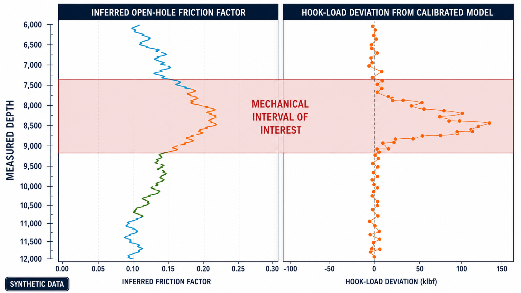
SPE-191426 describes automatically fitting open-hole friction factors against measured hook-load behavior at different measured depths.[1]

This turns friction from one constant input into something closer to a depth-dependent diagnostic signal.

Instead of asking:

What friction factor best describes the whole well?

we can ask:

What friction factor is required for the model to reproduce the measured behavior at this depth?

Then:

How does that inferred value change as the string moves through the hole?

That second question is often more operationally interesting.

Depth-dependent calibration can reveal intervals where measured mechanical behavior requires more drag than the surrounding hole.

Calibration Turns Routine Trips Into Experiments

Every trip contains mechanical information.

When the string is moving:

• the direction is known,
• depth is known,
• hook load is measured,
• trajectory is known,
• drillstring configuration is known or can be retrieved.

That creates repeated opportunities to compare:

$$ \text{Measured Mechanical Response} $$

with

$$ \text{Modeled Mechanical Response} $$

A real-time calibration system can therefore treat routine trips as repeated field experiments.

During trip out:

• pick-up behavior constrains the mechanical model.

During trip in:

• slack-off behavior provides another constraint.

During rotation off bottom:

• torque adds another independent observation.

As the operation progresses, the model gains more evidence about the actual well.

This is fundamentally different from running one pre-job T&D sensitivity table and assuming it remains valid for the rest of the well.

Rig State Is What Makes the Data Usable

The torque-and-drag equations depend on the mechanical condition being modeled.

A hook-load point collected during:

• pick-up,
• slack-off,
• rotation,
• a connection,
• reaming,
• static conditions,

cannot simply be thrown into the same calibration dataset.

The observations represent different physical states.

SPE-191426 explicitly relied on rig-state classification to identify conditions such as:

• pick-up,
• slack-off,
• rotating off bottom,
• and connections

for appropriate use in calibration.[1]

This illustrates why operational-state detection is so important in automated drilling analytics.

Raw data says:

Hook Load = 438 klbf

Context says:

Hook Load = 438 klbf while tripping out at this depth with this drillstring configuration.

Only the second statement is useful for friction calibration.

Real-time calibration requires selecting measurements generated under the physical state represented by the model.

Filtering Too Aggressively Can Remove the Event You Want to Find

Cleaning real-time data is necessary.

But filtering creates its own risk.

Suppose hook load contains a short-lived but genuine overpull.

A strong averaging routine may smooth that peak into an ordinary-looking data point.

The cleaned dataset looks better.

The mechanically important event disappears.

SPE-191426 describes iterations of the field implementation in which averaging reduced visibility of the full overpull magnitude. Removing that averaging preserved more of the actual event while other irrelevant observations continued to be filtered.[1]

This is a useful general lesson for drilling analytics:

Noise reduction and event preservation are competing objectives.

A filter appropriate for estimating a slowly varying friction baseline may be inappropriate for detecting:

• overpull,
• pressure spikes,
• vibration events,
• or other transient dysfunctions.

Filtering that improves a baseline estimate can also suppress the transient mechanical event the surveillance system is intended to detect.

A Friction Factor Is an Inference, Not a Direct Sensor Measurement

This distinction matters.

There is no surface sensor on the rig labeled:

Open-Hole Friction Factor = 0.27

Friction factor is inferred.

The model asks:

What value of friction would make the predicted hook load best reproduce what the rig actually measured?

That makes friction factor a model-dependent estimate.

Its quality depends on the quality of:

• trajectory,
• string description,
• buoyancy,
• mud weight,
• block-weight offset,
• measured hook load,
• state classification,
• and the mechanical assumptions of the model.

A calibrated friction-factor trend is therefore valuable.

But it should not be interpreted with more certainty than the inputs support.

The appropriate language is:

The observed mechanical response is consistent with a higher required friction factor in this interval.

rather than:

The physical coefficient of friction at 13,500 ft is exactly 0.31.

That distinction keeps the engineering interpretation grounded.

Model Residuals May Be More Informative Than the Fitted Parameter

Another way to interpret the system is to examine the residual:

$$ R = HL_{\mathrm{measured}} - HL_{\mathrm{modeled}} $$

where (HL) is hook load.

If the calibrated model normally reproduces trip-out hook load closely, but measured hook load suddenly exceeds the modeled response by 30 klbf, that residual may be more immediately useful than asking what single friction factor would make the point fit.

Why?

Because a localized residual can represent:

• a tight spot,
• accumulated cuttings,
• ledge interaction,
• temporary pack-off tendency,
• wellbore geometry effects,
• or another transient mechanical condition.

Forcing every abnormal observation into a new friction factor can turn an event into a calibration change.

Sometimes the correct conclusion is:

The baseline model remains valid, but the well has produced an abnormal mechanical event.

This leads to an important distinction:

Calibration

updates the normal model.

Surveillance

detects departures from the normal model.

Those functions should work together without becoming the same thing.

Overpull Is Meaningful Relative to an Expected Baseline

Consider two hook-load measurements:

450 klbf

and

470 klbf

Which is the overpull?

There is no answer without context.

At one depth, modeled pick-up weight may be 430 klbf.

At another, it may already be 465 klbf.

The meaningful quantity is not absolute hook load.

It is something closer to:

$$ \Delta HL = HL_{\mathrm{measured}} - HL_{\mathrm{expected}} $$

That is why calibrated torque-and-drag models are powerful for event detection.

The model supplies a mechanical baseline that changes with:

• depth,
• trajectory,
• drillstring configuration,
• and frictional conditions.

The surveillance logic can then evaluate whether the actual measurement departs unusually from that baseline.

SPE-191426 applied this concept to identifying probable overpull and underpull events while tripping.[1]

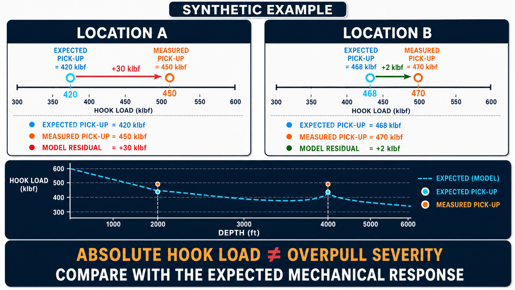
Mechanical events are best interpreted as departures from a depth-dependent expected response rather than by absolute hook load alone.

One Difficult Interval Can Persist Across Multiple Runs

A particularly useful application of real-time T&D is comparing mechanical behavior across successive BHA runs.

Suppose one trip encounters abnormal overpull near:

12,000 ft MD

A later cleanout run again shows unusual behavior near the same depth.

That recurrence tells the engineer something different from one isolated hook-load spike.

The problematic behavior may be associated with the hole rather than merely with one transient rig action.

SPE-191426 reports this kind of repeated depth-localized behavior in its field case.[1]

That is where real-time mechanical surveillance becomes more than an alarm system.

It becomes a way of building memory about the wellbore.

The question changes from:

Was there an overpull?

to:

Are we repeatedly seeing abnormal mechanical behavior in the same interval?

That information can influence:

• subsequent trips,
• cleanout decisions,
• reaming strategy,
• casing-running expectations,
• and risk assessment.

The Current BHA Run Can Inform the Future Casing Run

The mechanical information learned while drilling has value later in the well.

If calibrated trips repeatedly identify:

• elevated inferred friction,
• recurring overpull,
• or difficult depth intervals,

those observations can inform expectations for casing.

SPE-191426 extended the real-time modeling workflow to a subsequent production-casing run and compared casing behavior against the mechanical trends learned earlier in the well.[1]

This is an important idea.

The value of a calibrated T&D model is not limited to explaining what is happening now.

It can preserve information from one operation for use in the next one.

That creates a continuous workflow:

Drilling / BHA trips

→ learn mechanical response

→ identify troublesome intervals

→ update hole understanding

→ inform cleanout or casing strategy

This is much stronger than generating a new offline T&D spreadsheet each time the operation changes.

Mechanical information learned from drilling and tripping can be carried forward into later hole-conditioning and casing-running decisions.

A Practical Real-Time Calibration Workflow

A defensible workflow might look like this.

1. Build the physical model

Load:

• directional surveys,
• drillstring components,
• casing geometry,
• BHA,
• mud weight,
• pipe properties.

2. Establish the hook-load baseline

Calibrate or verify:

• block weight,
• effective drillpipe weight.

Do this before interpreting systematic disagreement as friction.

3. Classify the operation

Identify data corresponding to:

• trip out,
• trip in,
• rotation off bottom,
• connections.

Discard or separately handle data generated under incompatible conditions.

4. Fit baseline friction

Use appropriate trip-in, trip-out, and rotating observations to determine which friction factors best represent normal measured behavior.

5. Evaluate calibration stability

Ask:

• Does the inferred friction remain reasonably consistent?
• Does it change smoothly?
• Is one interval forcing an implausible fit?

6. Monitor residuals

Compare measurements with the calibrated baseline.

Look for:

• excessive positive hook-load deviation,
• excessive negative deviation,
• erratic response,
• repeated localized anomalies.

7. Separate baseline change from transient event

A persistent shift may justify recalibration.

One localized overpull may be an operational event rather than a new normal friction factor.

8. Preserve depth-localized learnings

Record intervals that repeatedly show:

• overpull,
• underpull,
• elevated required friction,
• or erratic mechanical response.

9. Reuse the information

Apply what was learned to:

• subsequent BHA trips,
• cleanout planning,
• reaming,
• casing-running forecasts.

Measured trip-out hook load agrees with the calibrated model over most of the well, while the zoomed difficult interval and synchronized trip view preserve the localized elevated response for engineering review.

What Real-Time T&D Does Not Eliminate

Automation does not remove uncertainty.

A soft-string model still contains assumptions.

Friction factor is still inferred.

Survey quality still matters.

String descriptions can still be wrong.

Hole geometry may differ from the nominal bit diameter.

Cuttings beds, ledges, keyseats, and local borehole features are not necessarily represented explicitly.

Sensor quality can still degrade.

And a model calibrated to one mechanical regime may not remain valid indefinitely.

A mature implementation should therefore expose enough evidence for the engineer to understand:

• what was measured,
• what the model predicted,
• what was calibrated,
• and where the two no longer agree.

The objective is not to make the physics invisible.

It is to remove repetitive manual work while preserving engineering interpretability.

The Most Valuable Output May Not Be the Friction Factor

It is tempting to think the end product of real-time T&D is a continuously updated number:

FF = 0.24

But that is probably not the most useful output.

The more valuable information may be:

• the model normally matches the well,
• this interval repeatedly departs from the baseline,
• the required drag increased here,
• the behavior improved after cleanout,
• this same interval was troublesome on the prior trip,
• and casing is likely to encounter the same mechanical challenge.

In that sense, friction factor is a tool.

The real product is mechanical situational awareness.

A calibrated model gives surface measurements a reference.

Without that reference, hook load is only a number.

With it, the engineer can begin asking:

Is this response normal for this depth and configuration?

Has the hole changed?

Is the anomaly localized?

Did the cleanout improve the mechanical condition?

What does this imply for the next operation?

That is the transition from running torque-and-drag calculations to using torque and drag as a real-time drilling intelligence system.

---

References

1. Shahri, M., Wilson, T., Thetford, T., Nelson, B., Behounek, M., Ambrus, A., D'Angelo, J., and Ashok, P. Implementation of a Fully Automated Real-Time Torque and Drag Model for Improving Drilling Performance: Case Study. SPE-191426-MS, SPE Annual Technical Conference and Exhibition, Dallas, Texas, 2018.