A tortuosity metric measures a sampled trajectory, not the physical wellbore independently of its survey. Change the station spacing and the calculation sees different geometric information, even though the hole has not changed. Any BHA or well comparison must therefore control survey resolution and preserve the distinction between measured and interpolated stations.
A survey is a sampled trajectory
A wellbore trajectory is continuous. A conventional directional survey is not. It consists of discrete observations along measured depth:
- measured depth,
- inclination,
- azimuth.
The trajectory between those stations is reconstructed mathematically, commonly using the minimum curvature method. This distinction matters. The survey does not contain every local variation in the physical wellbore. It contains the variations that can be observed at the locations where measurements were taken. Consider a hypothetical lateral that contains several small directional oscillations. A high-resolution survey might contain enough points to reveal each one. A conventional survey with stations approximately one stand apart may see only some of them. A still coarser representation could connect points on either side of several local variations and effectively hide them from the trajectory calculation.
The physical path did not become smoother. The measured representation became smoother.
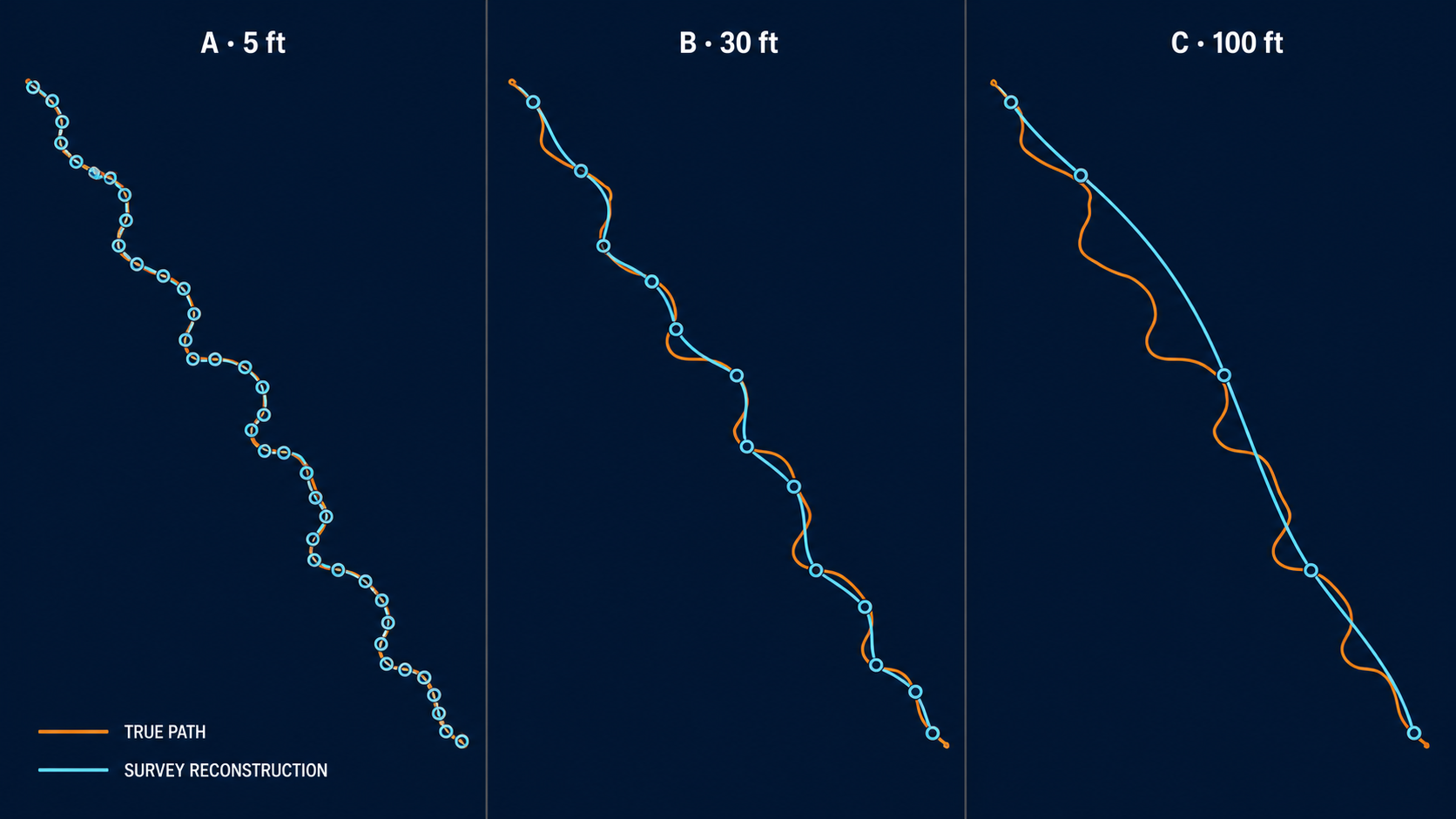
As survey spacing increases, local trajectory features can disappear from the sampled representation even though they remain in the actual wellbore.
The tortuosity approach evaluated in SPE-196020 considers two geometric characteristics of turns.[1]
| Characteristic | Meaning | Resolution effect |
|---|---|---|
| Frequency | Number of identified directional turns | Higher-resolution trajectories can expose turns hidden by wide station spacing. |
| Sharpness | Difference between the path through a turn and the direct path between its endpoints | Depends on the locations and geometry of the sampled points. |
Sharpness can be represented by comparing:
- the arc length through a turn,
- with the chord length connecting its endpoints.
For a nearly straight interval, the two distances are almost equal. For a sharper or more complicated turn, the path along the curve becomes longer relative to the straight-line connection. Together, frequency and sharpness describe how often the path changes direction and how significant those changes are.
What SPE-196020 demonstrated
The particularly useful part of SPE-196020 is that the authors did not merely speculate that resolution might matter. They tested it. The study used five gyro surveys originally available at approximately 1-ft resolution.[1] Those trajectories were progressively downsampled by removing survey points, producing representations with intervals ranging from very high resolution to intervals as large as approximately 120 ft. The tortuosity calculation was then repeated on each representation. That creates an unusually clean experiment. The wellbore stays the same. The underlying high-resolution survey stays the same. Only the number and spacing of points provided to the calculation changes.
If the tortuosity metric were completely independent of survey resolution, the calculated result should remain essentially unchanged. It did not. The calculated tortuosity varied as survey interval changed.[1] The behavior was also not as simple as assuming:
More survey points always produce proportionally more tortuosity.
The interaction between the number of identified turns and the geometric severity of those turns created more complicated behavior. This is exactly why survey resolution deserves attention before tortuosity values are compared across wells.
Why a universal correction is unsafe
If a KPI changes systematically with survey interval, the obvious data-science response is to fit the spacing relationship, remove the trend, and compare corrected values.
SPE-196020 tested a version of this idea.[1] For the specific dataset examined, removing general trends reduced the variation in tortuosity across survey intervals by approximately 50%. That sounds encouraging. But the authors explicitly cautioned against treating the correction as a general solution.[1] The reason is fundamental. The difference between a 30-ft survey and a 100-ft survey is not simply a scale difference. The lower-resolution survey has actually lost information about the trajectory. A linear correction can adjust a number. It cannot reconstruct geometric features that were never sampled.
That is why the paper ultimately argues that using reasonably consistent survey intervals is preferable, where possible, to relying on a universal correction factor.[1] This principle applies to many drilling KPIs: Normalization works best when the measurement processes are fundamentally comparable. It cannot always repair missing information.
Interpolation does not restore lost geometry
Once inconsistent survey spacing is recognized, resampling to a common interval seems like an obvious solution. Sometimes that helps; sometimes it only creates interpolated points between sparse measurements. The key distinction is whether the operation standardizes existing information or implies information that was never measured.
SPE-196020 found that resampling an already consistently sampled lateral did not necessarily improve the agreement with higher-resolution reference data.[1] One reason was point placement. A newly generated regular grid can fall at locations that miss geometric features captured by the original stations. Another reason is the trajectory reconstruction itself. The minimum curvature method produces a smooth mathematical path between survey stations. When sparse data are interpolated onto a new grid, that reconstructed path can appear smoother than the underlying high-resolution trajectory. The important distinction is More rows in a resampled dataset do not mean more measured information.
If a 100-ft survey is interpolated to 10-ft spacing, it now contains ten times as many rows. It does not contain ten times as much directional information.
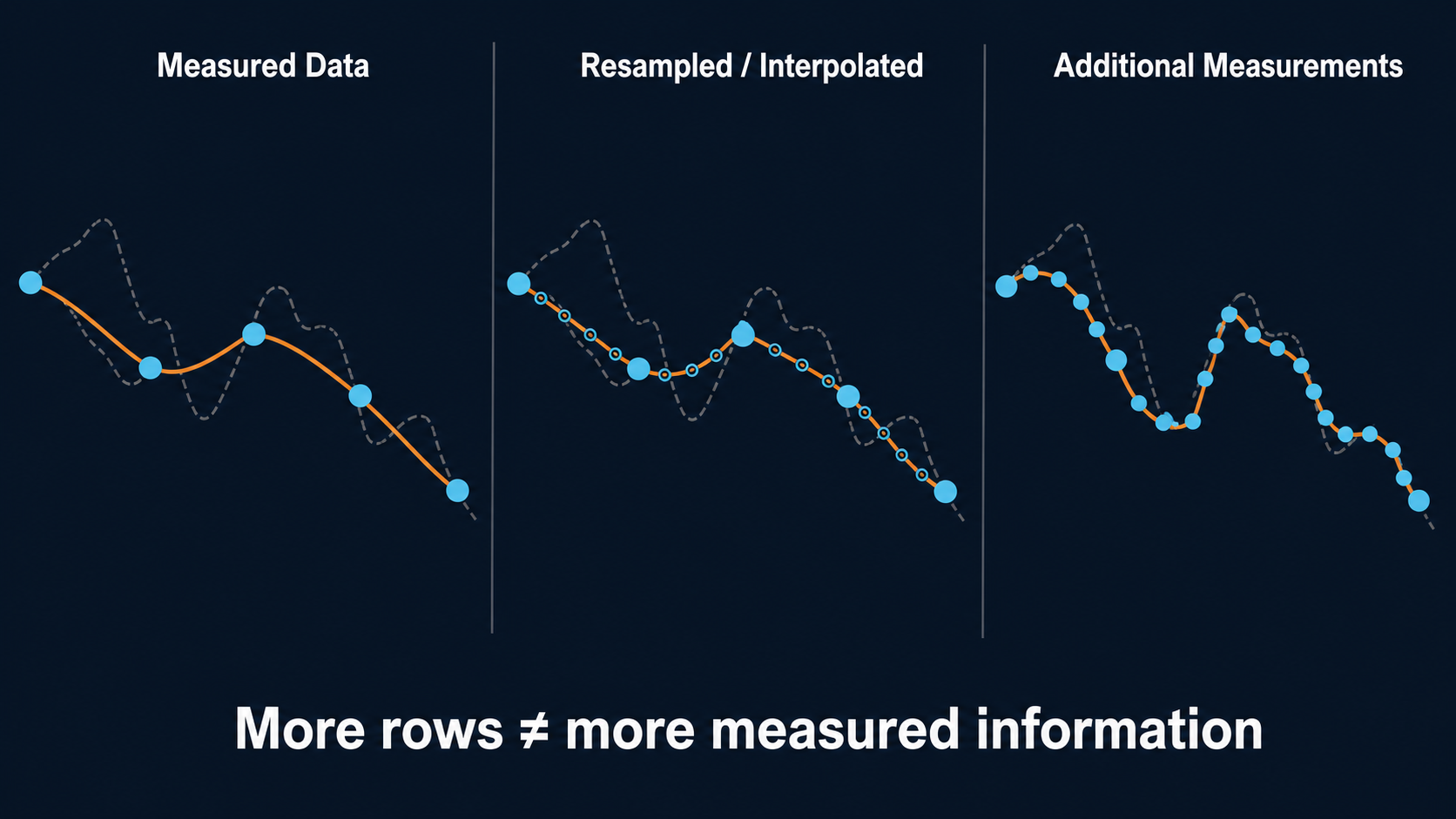
Resampling can standardize a dataset, but it cannot recreate trajectory information that was never measured.
Control the comparison and metric provenance
Once a tortuosity function exists in software, it is easy to calculate the value for every well in a database. That can create a false sense of comparability. A more defensible analytics workflow should store supporting information with the metric, including:
- section analyzed,
- survey source,
- median survey interval,
- minimum and maximum interval,
- interval variability,
- whether the data were resampled,
- resampling method,
- whether the survey is conventional or high resolution,
- and the tortuosity formulation used.
Then the tortuosity number has provenance. Without that information, a fleet-wide ranking can accidentally become a ranking of survey practices rather than just wellbore quality.
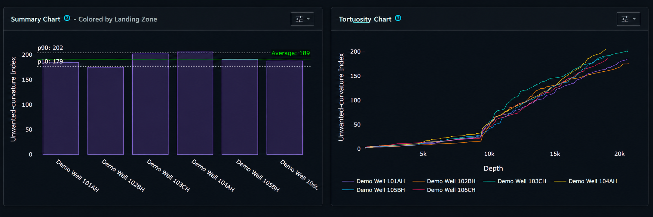
DrillingMetrics tortuosity views compare unplanned-curvature index across wells and depth.
Another useful observation from SPE-196020 was the difference between whole-well and lateral-only analysis.[1] The whole well contains distinctly different geometric regimes:
- vertical,
- build,
- potentially tangent,
- landing,
- lateral.
These sections often have different planned curvature and different survey practices. Combining them into one metric can therefore mix:
- intended geometry,
- directional execution,
- and measurement-resolution differences.
For BHA performance analysis, a section-specific comparison is often more defensible. A lateral BHA should generally be evaluated against other comparable lateral intervals. A curve BHA should be evaluated with consideration for the planned build geometry. This also connects to the distinction between:
- planned tortuosity,
- as-drilled tortuosity,
- and unplanned tortuosity.
A well that intentionally builds at a high rate is geometrically curved. That does not mean the directional execution was poor. The useful metric depends on the engineering question being asked.
Rules for fair BHA and well comparisons
There is no universal rule that every trajectory must be resampled. The source study argues against unnecessary resampling where survey intervals are already reasonably consistent.[1] For a fair comparison:
| Step | Practice |
|---|---|
| Inspect spacing | Plot or summarize the actual station intervals, not only their average. |
| Define the section | Avoid mixing survey practices and planned geometry from vertical, curve, and lateral sections. |
| Test materiality | Small interval differences may have little effect; large differences deserve attention. |
| Preserve measurements | Do not replace measured stations with interpolated points merely to make a uniform table. |
| Downsample deliberately | If necessary, downsample the higher-resolution dataset so both contain similar geometric information; this cannot restore information missing from the lower-resolution survey. |
| Preserve provenance | Store original and normalized results separately with the transformation history. |
Related technical resources
- Two Clocks, One Well: Modeling Time- and Depth-Indexed Data
- Practical Considerations in Offset-Well Benchmarking
- Comparing Slide and Rotate Performance Without Misleading Averages
References
- Shahri, M., James, M., Vasicek, A., De Napoli, R., White, M., Behounek, M., D'Angelo, J., Ashok, P., and van Oort, E. Case Studies: Optimizing BHA Performance by Leveraging Data and Advanced Modeling. SPE-196020-MS, SPE Annual Technical Conference and Exhibition, Calgary, Alberta, Canada, 2019.