When to Trust a Statistical Drilling Benchmark—and When Not To

A benchmark becomes useful only when its underlying population, measurement method, sample size, weighting, and drilling context support the comparison being made. More historical data does not automatically make the benchmark more reliable.

Suppose a drilling-performance dashboard shows:

Median rotary ROP: 215 ft/hr

and:

P75 rotary ROP: 248 ft/hr

Those numbers look authoritative.

But before using:

248 ft/hr

as a target for the current well, several questions matter.

How many wells produced the benchmark?

Which formations were included?

Were all observations drilled with comparable:

• hole size,
• bit,
• BHA,
• mud system?

Was sliding removed?

Are the observations:

• one-second sensor samples,
• stands,
• BHA runs,
• wells?

Did one exceptionally long well contribute most of the data?

Were poor-performing wells excluded?

Was ROP calculated consistently across the fleet?

Were older wells drilled with materially different technology?

Those questions determine whether the benchmark is:

strong engineering evidence

or merely:

a precisely calculated statistic.

That distinction is important.

Modern drilling databases can contain millions or billions of sensor observations.

That makes it easy to create numbers with impressive statistical precision.

But the number of database rows is not the same as the number of independent drilling experiences represented.

And a benchmark created from the wrong population can become more confidently wrong as more data is added.

The central question is therefore not:

Do we have enough data?

It is:

Do we have enough relevant, comparable, independently informative data to support the engineering comparison we want to make?

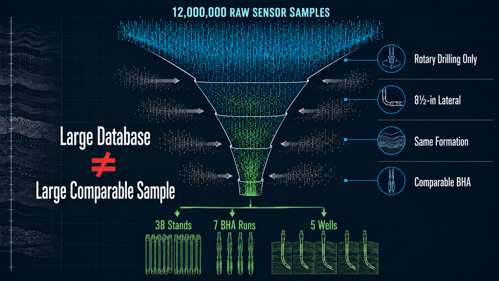
A large database can collapse to a small comparable sample once drilling mode, hole section, formation, and BHA context are applied.

A Benchmark Is a Summary of a Population

A benchmark might be:

• average ROP,
• median connection time,
• P75 slide ROP,
• P90 trip speed,
• median MSE,
• best-performing BHA,
• top-quartile well duration.

Every one of those statistics summarizes some population.

That population must be defined before the number can be interpreted.

For example:

Median ROP = 215 ft/hr.

Median of what?

Possibilities include:

• every recorded sensor sample,
• rotary drilling samples,
• stands,
• one specific formation,
• one BHA family,
• all laterals in the field.

The statistic does not contain that definition by itself.

The benchmark is therefore incomplete without its denominator.

Statistical Precision and Engineering Relevance Are Different

Imagine two benchmarks.

Benchmark A

Based on:

40 comparable lateral stands

from:

• the same formation,
• same hole size,
• similar bit/BHA configuration.

Benchmark B

Based on:

50,000 stands

from:

• several formations,
• multiple hole sizes,
• different BHA systems,
• several years of operating practices.

Benchmark B has far more data.

It may also be far less relevant to the current question.

This reveals two different concepts.

Statistical precision

How stable is the estimate within the population that produced it?

Engineering relevance

Does that population represent the drilling condition we are trying to evaluate?

A benchmark can have excellent statistical precision and poor engineering relevance.

In operational drilling, relevance frequently matters more.

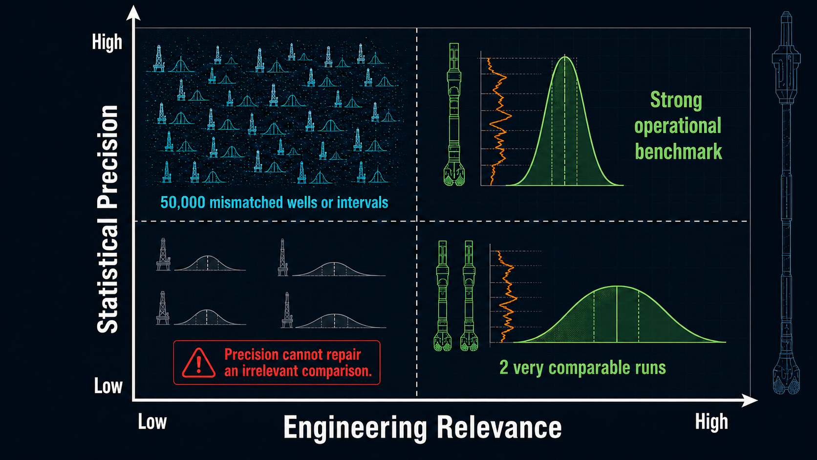
Statistical precision and engineering relevance are separate properties. A very stable estimate can still answer the wrong engineering question.

Sensor Samples Are Not Independent Wells

Suppose a rig records at:

1 Hz.

One hour of drilling provides:

$$3600$$

sensor observations.

Ten hours provides:

$$36,000$$

observations.

Has the system experienced 36,000 independent drilling conditions?

Of course not.

Adjacent samples are strongly related.

The bit is:

• in the same well,
• often in the same formation,
• using the same BHA,
• under nearly the same parameters.

This is a classic problem in time-series statistics.

Nearby observations are correlated.

Counting every sensor sample as though it were an independent experiment creates an illusion of sample size.

The Natural Unit Depends on the Question

A drilling dataset is hierarchical.

Conceptually:

$$Samples \rightarrow Intervals \rightarrow Stands \rightarrow BHA\ Runs \rightarrow Wells \rightarrow Rigs$$

Different questions require different analytical units.

Question

What is typical instantaneous rotary torque?

Sensor or short-interval observations may be appropriate.

Question

How does ROP vary between stands?

The stand becomes a useful unit.

Question

Which BHA configuration performs better?

BHA runs become important.

Question

Did one drilling program outperform another?

The number of independent wells may matter much more than the number of one-second samples.

A useful benchmark should identify the unit on which the comparison is based.

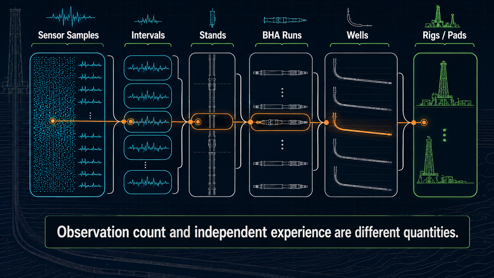
Observation count and independent drilling experience are different quantities. The evidence hierarchy should remain visible.

Ten Million Samples From One Well Are Still One Well

This point deserves emphasis.

Suppose:

Dataset A

10 million sensor observations

from:

one well.

Dataset B

500,000 observations

from:

ten wells.

For understanding detailed transient behavior, Dataset A may be extremely valuable.

For determining whether performance generalizes across wells, Dataset B may contain more independent evidence.

The larger raw dataset does not automatically provide the stronger benchmark.

This is why drilling analytics benefits from preserving the hierarchy between:

• samples,
• stands,
• wells.

Large Historical Databases Still Need Filtering

SPE-196020 analyzed historical lateral BHA performance across more than 300 BHA runs.

That size makes the dataset powerful.

But the study did not simply calculate one global ROP average.

The analysis included metadata such as:

• BHA specifics,
• directional-drilling provider,
• mud properties,
• RSS versus steerable systems,
• tortuosity.

That context allowed engineers to investigate why particular runs occupied:

• high-performance,
• low-performance

parts of the dataset.

The lesson is:

large databases become valuable when their metadata allows meaningful populations to be defined.

Not when everything is averaged together.

The Best Benchmark Population Is Usually Narrower Than the Database

Imagine a database containing:

300 lateral BHA runs.

The current well uses:

• 8½-in. hole,
• steerable motor,
• Formation B,
• oil-based mud,
• rotary drilling.

After filtering:

300 runs

may become:

Then filter for comparable formation:

Then comparable BHA architecture:

The engineeringly meaningful sample may be much smaller than the original database.

That is not necessarily a problem.

It is often a sign that the benchmark is becoming more relevant.

But Filtering Too Aggressively Creates Another Problem

Now continue filtering.

Same:

• bit model,
• motor bend,
• stabilizer spacing,
• exact mud weight,
• exact WOB range,
• exact RPM range.

The 18 runs become:

2.

The comparison is highly specific.

The sample is weak.

This creates a fundamental tradeoff.

Broader population

More data
Less comparability

Narrower population

Better comparability
Less data

A good statistical drilling benchmark finds a useful balance.

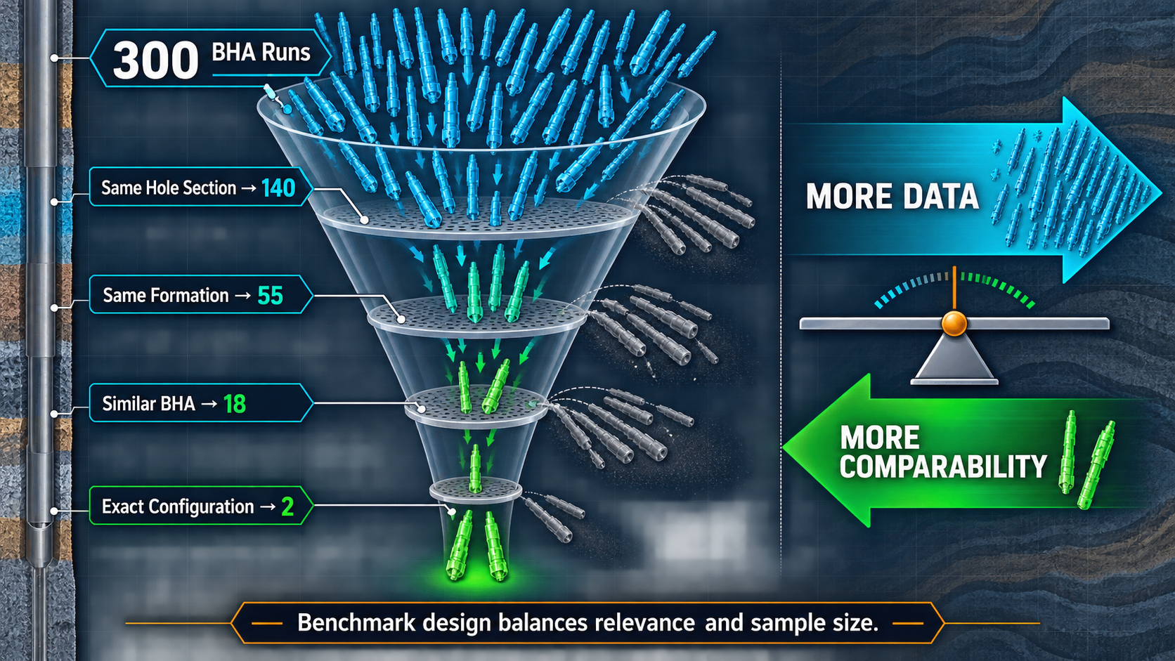
Each additional context filter improves matching but reduces available evidence. Benchmark design must balance comparability against statistical uncertainty.

There Is No Universal Minimum Number of Wells

Engineers often ask:

How many wells do I need before the benchmark is reliable?

There is no universal answer.

It depends on:

• variability,
• effect size,
• measurement quality,
• independence,
• similarity of wells,
• question being asked.

Five extremely comparable wells can provide useful operational guidance.

Five wells cannot usually prove that a modest difference between two technologies is universally real.

The field papers themselves illustrate this caution.

SPE/IADC-194184 compared drilling performance across 25 wells on four rigs.

Even with 25 wells, the authors explicitly cautioned that the dataset remained limited for hard conclusions and that many other variables affected the observed ROP differences.

That is exactly the right statistical instinct.

Performance Attribution Is Harder Than Performance Description

Suppose:

Program A

Average ROP:

190 ft/hr

Program B

Average ROP:

210 ft/hr

We can describe:

Program B had higher observed average ROP.

Can we say:

The new BHA caused a 20-ft/hr improvement?

Not yet.

Other changes might include:

• crew,
• formation,
• bit,
• mud,
• directional requirement,
• operating parameters.

This distinction is fundamental.

Descriptive benchmark

What happened?

Causal attribution

Why did it happen?

Historical drilling datasets are usually much stronger at the first than the second.

A Benchmark Should Not Pretend to Be an Experiment

In a controlled experiment:

one factor changes while others remain comparable.

Drilling operations rarely work that way.

From one well to the next:

• geology changes,
• crew changes,
• bit changes,
• BHA changes,
• operational learning accumulates.

Therefore:

$$Performance_{new} - Performance_{old}$$

cannot automatically be attributed to:

$$Technology\ Change$$

The benchmark is observational evidence.

It should be interpreted accordingly.

Formation Mix Can Reverse the Conclusion

Consider a hypothetical comparison between two rigs.

Rig A performs better in both formations.

Soft Formation

Rig A:

220 ft/hr

Rig B:

210 ft/hr

Hard Formation

Rig A:

140 ft/hr

Rig B:

130 ft/hr

Rig A is faster in both.

But now consider the formation mix.

Rig A

20% soft
80% hard

Overall:

$$0.20(220)+0.80(140) = 156\ ft/hr$$

Rig B

80% soft
20% hard

Overall:

$$0.80(210)+0.20(130) = 194\ ft/hr$$

The overall average suggests:

Rig B is dramatically faster.

Yet within each formation:

Rig A performs better.

This is a form of what statisticians call Simpson's paradox.

The direction of the aggregate comparison changes when the population mix is considered.

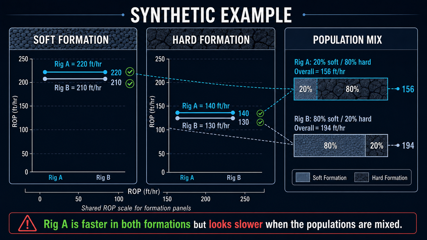
Synthetic example: Rig A is faster within both formations but appears slower after unequal formation populations are combined.

This Is Why Formation Normalization Matters

The aggregate benchmark answered:

What average ROP did each rig experience?

It did not answer:

Which rig performed better under comparable rock conditions?

Those are different questions.

The first may be useful for:

• actual well-delivery history.

The second is more useful for:

• operational-performance comparison.

The benchmark design should reflect the intended decision.

Drilling Mode Can Produce the Same Problem

The slide-versus-rotate article demonstrated another mixture effect.

A well with higher:

• rotary ROP,
• slide ROP

can still have lower blended lateral ROP if it is required to slide substantially more footage.

Thus:

$$Blended\ ROP$$

contains both:

• drilling-mode performance,
• mode mix.

Comparing wells without separating those components can rank directional requirement instead of drilling execution.

Weighting Determines the Question Being Answered

Suppose we have two stands.

Stand 1

100 ft at 200 ft/hr.

Stand 2

20 ft at 50 ft/hr.

The simple average of the two stand ROPs is:

$$\frac{200+50}{2} = 125\ ft/hr$$

But actual drilling time is:

$$100/200 + 20/50 = 0.9\ hr$$

and total footage is:

120 ft.

The effective section ROP is:

$$120/0.9 \approx 133\ ft/hr$$

Neither number is inherently wrong.

They answer slightly different questions.

Equal-weight stand average

What does the average stand-level ROP value look like?

Footage/time-derived section ROP

How quickly was the footage actually delivered?

Benchmark methodology should state which is being used.

Time Weighting Can Overrepresent Slow Drilling

Suppose raw 1-Hz samples are used to calculate an ROP distribution.

A slow stand takes longer.

It produces more samples.

A fast stand produces fewer samples.

Therefore a time-sampled distribution naturally gives more weight to slow drilling.

That may be appropriate if the question is:

What operating condition consumed most drilling time?

It may be inappropriate if the question is:

What ROP did a typical stand achieve?

This is a subtle but important analytical issue.

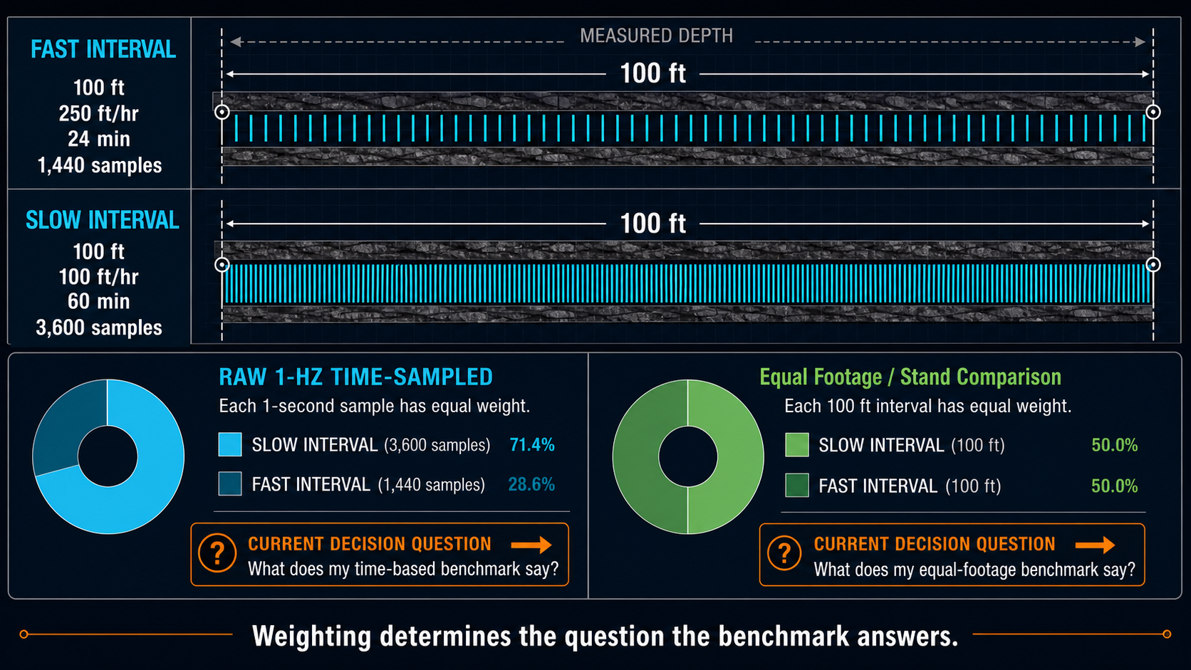
A slow interval contributes more time samples than an equal-footage fast interval, so the weighting scheme changes the question being answered.

Footage Weighting Can Answer a Different Question

A depth-binned dataset may give similar representation to equal footage intervals.

That can be useful for:

• formation benchmarking,
• lateral comparisons.

But it can underrepresent the amount of time consumed by slow intervals.

Again:

the correct weighting depends on the engineering question.

A benchmark should not hide its weighting scheme.

The Metric Itself Must Be Consistent

SPE-196020 provides an excellent example using tortuosity.

The study found that Tortuosity Index values could vary materially with:

• survey interval,
• consistency of survey spacing.

Therefore two identical physical wellbores could appear different analytically if the measurement resolution differed.

This is a crucial benchmarking lesson.

Before comparing the statistic, ensure that the statistic was measured the same way.

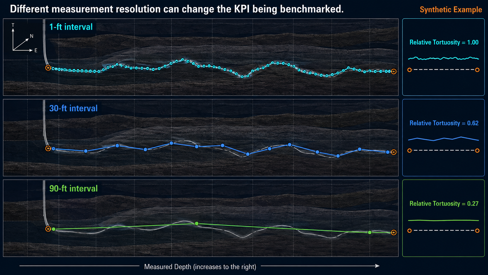
The same physical wellbore can produce different apparent tortuosity when survey spacing changes.

Metric Versioning Matters Too

Suppose historical ROP was calculated using one definition.

The current system uses another.

Or:

MSE v1

used surface RPM only.

MSE v2

includes estimated motor RPM.

The benchmark may now contain two different analytical definitions under one name.

This is not a statistical problem in the narrow sense.

It becomes one the moment those values are pooled.

A trustworthy historical benchmark should preserve:

• metric definition,
• filtering rules,
• algorithm version

where those differences materially affect interpretation.

The Best Wells Are a Biased Sample

Another common practice is:

Benchmark against the top five wells.

That can be useful operationally.

But it introduces selection bias.

The top wells may have benefited from:

• unusually favorable geology,
• new bits,
• easier directional requirement,
• exceptionally clean hole conditions.

Selecting only the winners removes the conditions that produced average or poor outcomes.

The resulting benchmark answers:

What has been achieved under the best observed combinations of circumstances?

It does not necessarily answer:

What should we reasonably expect on the current well?

Those are different uses.

A Top-Quartile Benchmark Is a Target, Not a Prediction

Suppose:

P75 rotary ROP:

240 ft/hr

The number can serve as:

• an aspirational performance reference.

It should not automatically be interpreted as:

The current well should drill at 240 ft/hr.

The current well may have:

• harder rock,
• greater lateral length,
• different BHA,
• more restrictive operating limits.

Percentiles describe the historical population.

They do not guarantee a future outcome.

The Benchmark Should Show Dispersion

Consider two formations.

Formation A

Median ROP:

200 ft/hr

P25:

190

P75:

210

Formation B

Median ROP:

200 ft/hr

P25:

130

P75:

270

The medians are identical.

The operational predictability is completely different.

This is why a useful benchmark often includes:

• median,
• percentiles,
• sample count,
• perhaps spread.

A single target value hides the uncertainty around it.

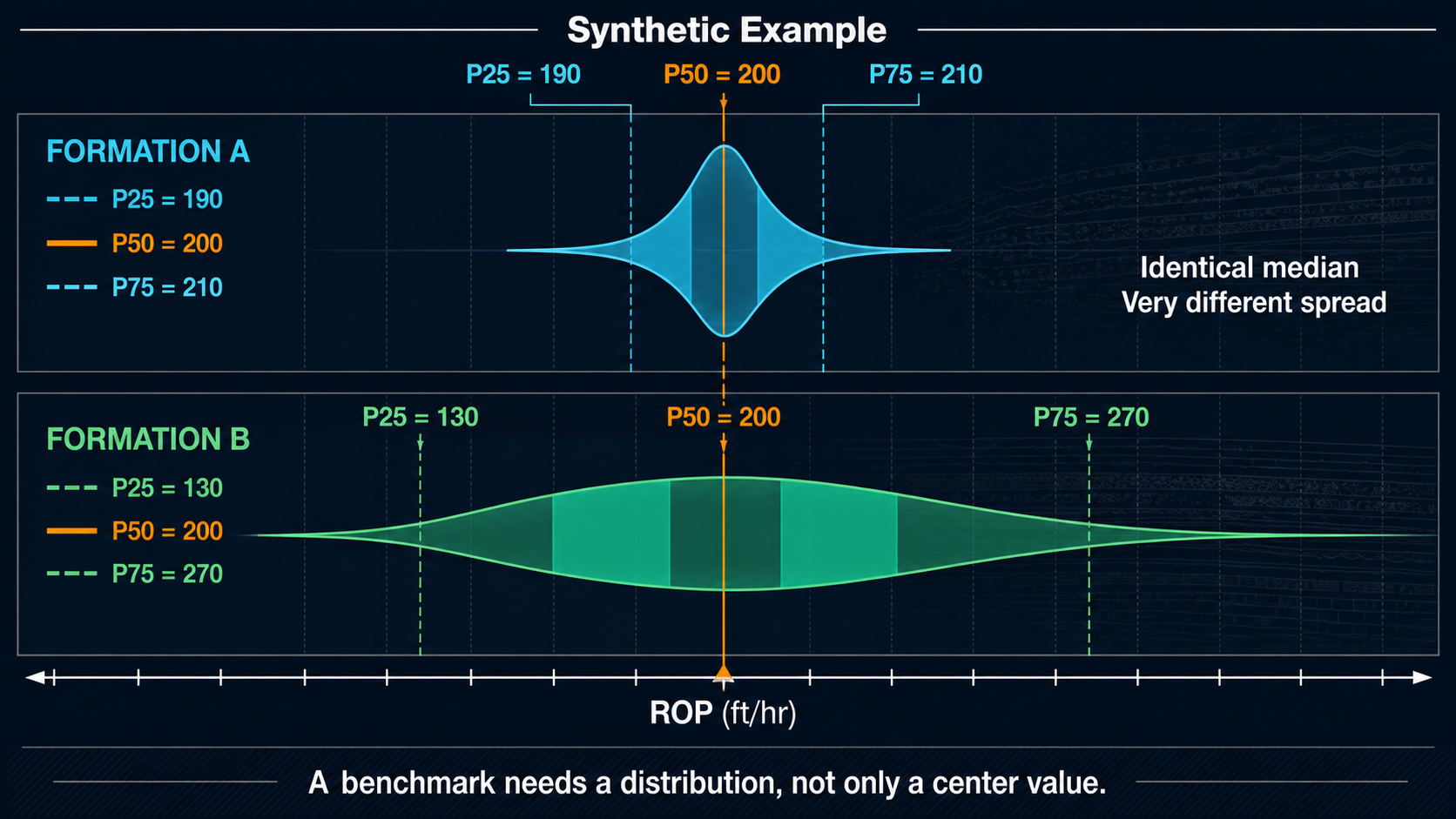
Identical medians can conceal radically different operational uncertainty.

Sample Count Should Accompany the Benchmark

Consider:

P75 ROP = 240 ft/hr

with:

n = 4 stands.

Now:

P75 ROP = 240 ft/hr

with:

n = 240 stands across 12 wells.

Those values should not create equal confidence.

Showing the sample count is one of the simplest ways to prevent overinterpretation.

But the count should identify the analytical unit.

For example:

• 240 stands,
• 12 BHA runs,
• 8 wells.

That is more informative than:

n = 86,417

when 86,417 refers to raw one-second samples.

Show the Number of Wells Too

Suppose a benchmark contains:

500 stands.

Sounds strong.

But 420 came from:

one well.

The benchmark may therefore reflect:

• one formation realization,
• one BHA,
• one crew,
• one bit run sequence.

A useful summary might show both:

Stands: 500

and:

Wells: 6

This exposes the hierarchy of the evidence.

One Rig Can Dominate the Fleet Benchmark

The same problem appears at fleet scale.

Suppose:

Rig A contributes:

60% of all observations.

Rigs B through F contribute the rest.

A fleet median may actually resemble:

Rig A's operating history

more than the fleet as a whole.

Depending on the question, it may be useful to:

• weight wells equally,
• weight rigs equally,
• display rig-specific distributions.

Again, weighting is part of benchmark design.

Repeated Success Matters More Than One Record Run

A record lateral proves:

the performance is possible.

It does not prove:

the performance is repeatable.

Those are different forms of evidence.

For operational planning, repeated:

• strong,
• stable,
• reproducible

performance may be more valuable than one extreme outlier.

This suggests distinguishing:

Best observed

What is the record?

Typical high performance

What does the strong-performance distribution look like?

Repeatable performance

How consistently does the system stay in that range?

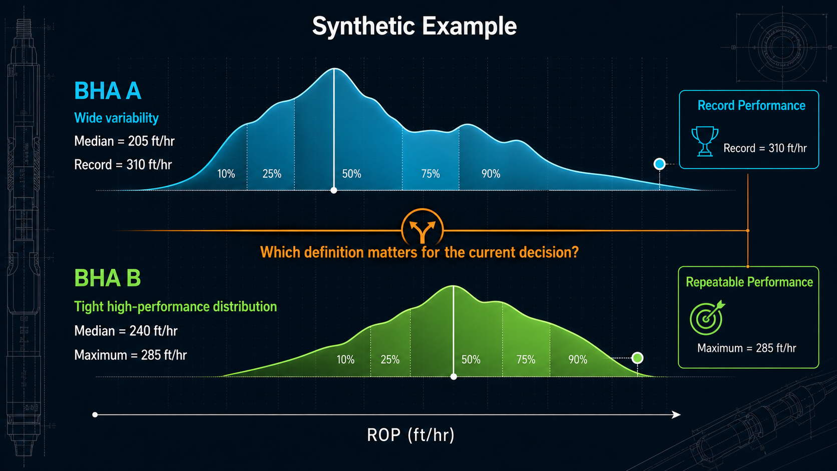
One extreme record demonstrates possibility; a tight high-performance distribution demonstrates repeatability.

Variability Is Part of Performance

Imagine two BHAs.

BHA A

Median rotary ROP:

220 ft/hr

wide spread:

120–300.

BHA B

Median:

210 ft/hr

tight spread:

190–230.

Which is better?

The answer depends on the operation.

If predictability matters:

BHA B may be highly attractive.

A benchmark that ranks only median or maximum performance misses this aspect.

ROP Ranking Can Conflict With Wellbore-Quality Ranking

SPE-196020 provides real field examples in which:

• ROP ranking,
• tortuosity ranking

do not align.

One well can drill faster but produce a less desirable wellbore-quality metric.

Another can drill more slowly while ranking much better for tortuosity.

Therefore:

benchmarking requires an objective.

Are we comparing:

• ROP,
• wellbore quality,
• total section delivery,
• NPT,
• MSE?

There may be no universal “best well.”

Benchmark Drift Is Real

A field evolves.

New:

• bits,
• motors,
• RSS systems,
• drilling practices,
• control systems

are introduced.

A benchmark containing wells drilled five years ago may represent:

historical capability

rather than:

current capability.

Old data is not necessarily useless.

It may still show:

• formation behavior,
• failure patterns,
• mechanical limits.

But performance targets may need recency context.

A benchmark should therefore consider:

Is the population technologically comparable to today's operation?

Learning Creates Another Confounder

Suppose a new BHA design is introduced.

The first few wells perform modestly.

Later wells perform better.

Did the BHA improve?

Or did crews learn how to operate it more effectively?

Possibly both.

This is one reason historical performance attribution is difficult.

SPE/IADC-194184 explicitly notes that drilling success depends on multiple factors, including crew performance and experience, making it difficult to attribute observed performance improvement solely to one advisory technology.

Current-Well Data Should Eventually Challenge the Historical Benchmark

Historical benchmarks are most valuable before the new interval has generated much evidence.

Once the current well drills several comparable stands, we now have:

local evidence.

Suppose historical P50 rotary ROP is:

200 ft/hr.

The current well consistently drills:

235 ft/hr

under stable conditions.

Should 200 remain the target simply because the historical database says so?

No.

The current well may have:

• a better bit,
• better BHA,
• different rock response.

SPE-186166 makes a similar point for drilling parameters: historical post-well analysis is useful as a starting point, but real-time data reflects the current drilling reality more directly.

A benchmark should initialize expectations.

It should not prevent them from being updated.

A Statistical Benchmark Should Have a Scope

Instead of displaying:

P75 ROP = 240 ft/hr

show something closer to:

Rotary ROP — P75: 240 ft/hr

Scope:

• 8½-in. lateral,
• Formation B,
• motor BHA family,
• last 12 comparable wells.

Evidence:

• 184 stands,
• 12 wells.

Now the statistic has engineering meaning.

A Useful Benchmark Card

A mature benchmark could conceptually show:

Metric

Rotary ROP

Population

Formation B
8½-in. lateral
Motor BHA

P25

185 ft/hr

P50

215 ft/hr

P75

242 ft/hr

Evidence

196 stands
11 BHA runs
8 wells

Recency

Last 18 months

Exclusions

Slide drilling
Connections
Known sensor-fault intervals

That is much more informative than:

Target ROP = 242.

A Practical Example

Suppose an engineer wants to compare two BHA configurations.

Historical database:

BHA A

70 stands
5 wells

Median rotary ROP:

215 ft/hr

BHA B

60 stands
4 wells

Median rotary ROP:

230 ft/hr

At first glance:

BHA B appears better.

Now stratify by formation.

Formation X

BHA A:

235 ft/hr

BHA B:

238 ft/hr

Nearly identical.

Formation Y

BHA A:

190 ft/hr

BHA B:

192 ft/hr

Again nearly identical.

Why was the aggregate median different?

BHA B happened to drill substantially more footage in:

Formation X.

The apparent BHA advantage largely disappears after normalization.

The original statistic was numerically correct.

The engineering interpretation was wrong.

That is the central risk of an unqualified benchmark.

A Practical Reliability Checklist

Before acting on a drilling benchmark, ask:

What exactly is the metric?

ROP?

MSE?

Connection duration?

What is the analytical unit?

Samples?

Stands?

Runs?

Wells?

What population produced it?

Formation?

Hole section?

BHA?

Drilling mode?

How much independent evidence exists?

How many:

• stands,
• runs,
• wells?

Is the measurement method consistent?

Same:

• calculation,
• units,
• filtering,
• survey resolution?

How is the data weighted?

By:

• time,
• footage,
• stand,
• well?

What is the spread?

Is performance:

• consistent,
• highly variable?

Is there selection bias?

Are we looking at:

• all wells,
• only the best?

Is the data still relevant?

Have:

• bits,
• BHAs,
• practices

changed materially?

Does the benchmark answer the decision being made?

A valid benchmark for one question may be inappropriate for another.

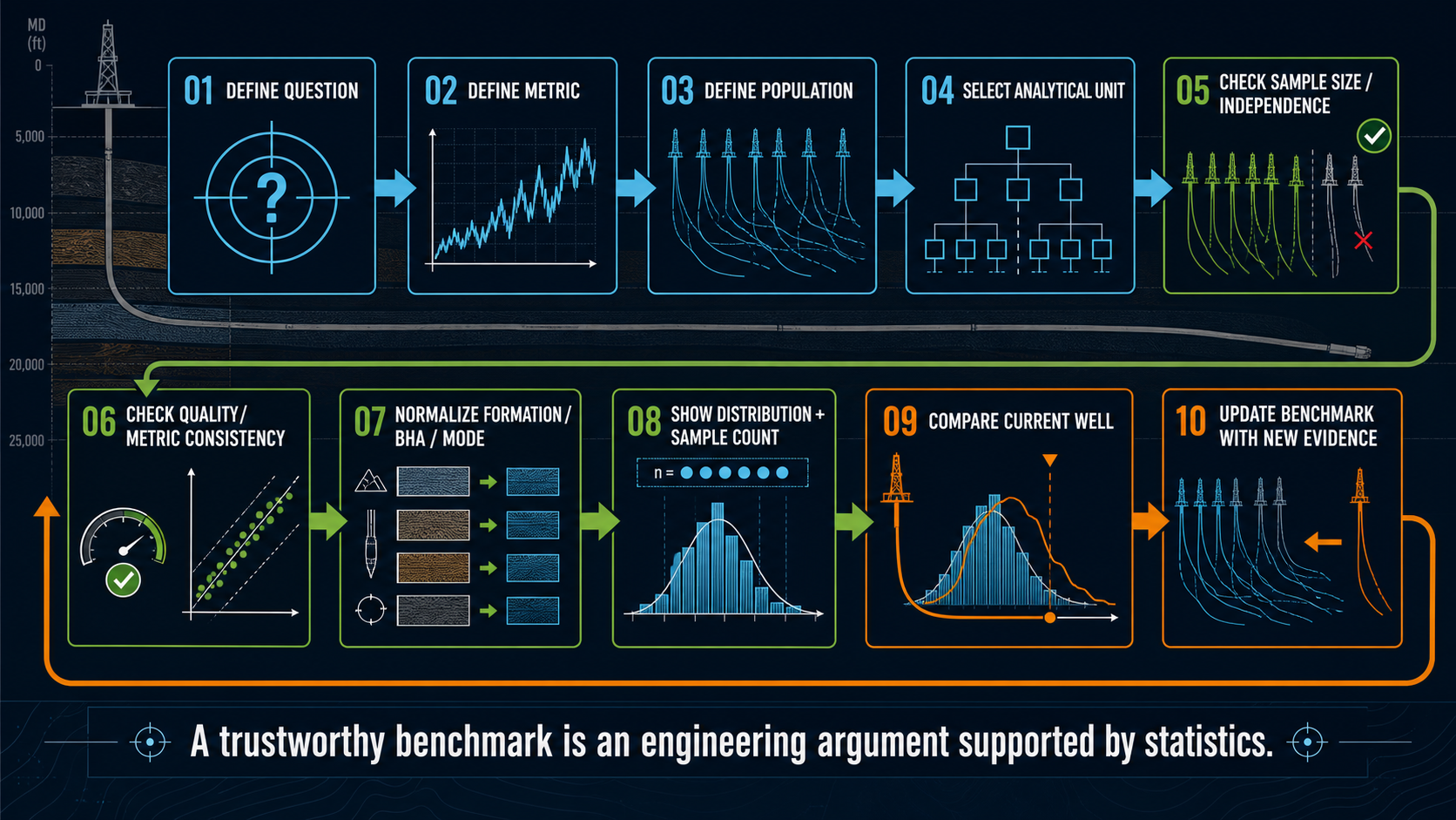
A trustworthy benchmark is built by defining the question, metric, population, analytical unit, consistency checks, and current-well update path.

Population Context in DrillingMetrics

The same ROP metric can tell a different story as the comparison population becomes more specific.

Broad well population

Includes overall well ROP across the available intervals.

Rotary-only population

Removes slide drilling and changes the operating-state mix.

Lateral rotary population

Restricts the comparison to rotary drilling in the lateral, making the population more relevant to that engineering question.

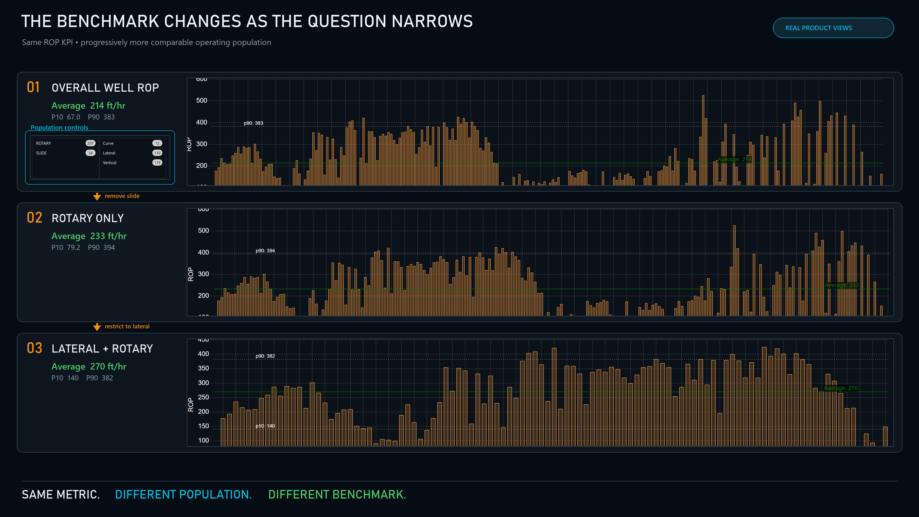
In these captured product views, the reported average changes from 214 to 233 to 270 ft/hr as the operating population narrows. This is a population change, not causal proof of improvement.

The filter progression demonstrates the article's core point:

the benchmark changes when the population becomes engineeringly comparable.

AIDE can add another layer by listing recent wells at the well level and grouping them by lease area. That context exposes which wells contribute to the comparison instead of presenting a benchmark without its population.

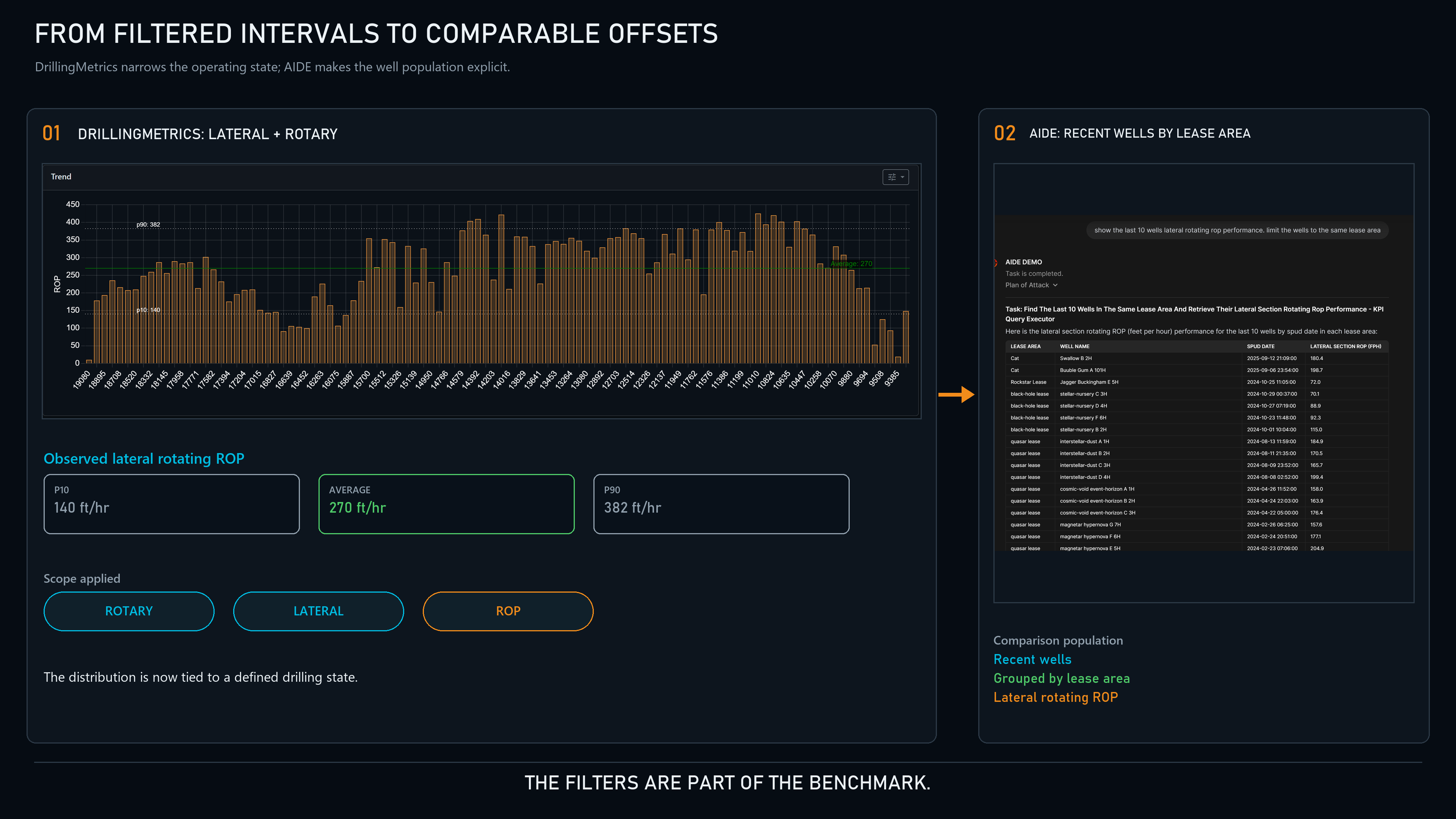
DrillingMetrics isolates a defined operating state; AIDE makes the recent well-level comparison population and lease-area grouping explicit.

What Makes a Benchmark Strong?

A strong drilling benchmark usually has several characteristics.

It is:

Well defined

The metric and population are explicit.

Comparable

Major operational and geological confounders are controlled or visible.

Sufficiently populated

There is enough independent evidence for the intended conclusion.

Consistently measured

The metric means the same thing throughout the dataset.

Transparent

The user can see:

• distribution,
• sample size,
• scope.

Current enough

The historical population still represents the equipment and process being evaluated.

Updateable

Current-well evidence can modify the expectation.

What Makes a Benchmark Weak?

Be cautious when:

One large well dominates the data

Raw sample count exaggerates evidence.

Mixed formations are averaged together

Population mix can reverse conclusions.

The metric changed over time

Historical and current values are not truly comparable.

Only top-performing wells are included

The result becomes an aspiration rather than an expectation.

The sample is tiny after filtering

The benchmark may be relevant but statistically unstable.

A descriptive comparison is treated as causal proof

Observed improvement does not prove one factor caused it.

The Benchmark Should Inform Judgment, Not Replace It

This is ultimately the purpose of historical drilling analytics.

A benchmark can tell the engineer:

• what has happened,
• how performance is distributed,
• what strong performance has looked like,
• how unusual current behavior is.

It cannot guarantee:

• what this well must do,
• why historical differences occurred,
• which single parameter created the result.

The strongest benchmark narrows the engineering uncertainty.

It does not pretend that uncertainty disappeared.

Conclusion

Modern drilling databases make it easy to calculate benchmarks.

The harder problem is deciding whether those benchmarks deserve to influence an operational decision.

A trustworthy benchmark requires more than:

lots of data.

It requires:

• a clearly defined metric,
• a relevant comparison population,
• meaningful analytical units,
• adequate independent observations,
• consistent measurement methodology,
• appropriate weighting,
• visibility into variability and sample size.

Perhaps the most important distinction is this:

A statistically stable benchmark can still be engineeringly wrong for the current well.

Millions of observations from mismatched conditions do not repair that problem.

Conversely, a smaller dataset of genuinely comparable wells may provide extremely useful evidence—provided its uncertainty is acknowledged.

Historical drilling data is therefore most powerful when it is treated neither as:

anecdote

nor:

ground truth.

It is evidence.

The engineering task is to determine:

which evidence is comparable, how much independent evidence exists, how variable it is, and whether it actually answers the question being asked.

That is when a drilling benchmark becomes something worth trusting.

---

References

1. Behounek, M., Millican, B., Nelson, B., Wicks, M., Rintala, E., White, M., Thetford, T., Ashok, P., and Ramos, D. Change Management Challenges Deploying a Rig-Based Drilling Advisory System. SPE/IADC-194184-MS, SPE/IADC International Drilling Conference and Exhibition, The Hague, Netherlands, 2019.

2. Shahri, M., James, M., Vasicek, A., De Napoli, R., White, M., Behounek, M., D'Angelo, J., Ashok, P., and van Oort, E. Case Studies: Optimizing BHA Performance by Leveraging Data and Advanced Modeling. SPE-196020-MS, SPE Annual Technical Conference and Exhibition, Calgary, Alberta, 2019.

3. Ambrus, A., Ashok, P., Chintapalli, A., Ramos, D., Behounek, M., Thetford, T. S., and Nelson, B. A Novel Probabilistic Rig Based Drilling Optimization Index to Improve Drilling Performance. SPE-186166-MS, SPE Offshore Europe Conference & Exhibition, Aberdeen, United Kingdom, 2017.

4. Behounek, M., Thetford, T., Yang, L., Hofer, E., White, M., Ashok, P., Ambrus, A., and Ramos, D. Human Factors Engineering in the Design and Deployment of a Novel Data Aggregation and Distribution System for Drilling Operations. SPE/IADC-184743-MS, SPE/IADC Drilling Conference and Exhibition, The Hague, Netherlands, 2017.